UGC NET MICRO ECONOMICS MATERIAL

CONCEPT OF DEMAND
The concept of demand was given by Alfred Marshall in 1890s in his
book “Principles of Economics”. According to him, the demand can
be represented by following words:
1. Desire
2. Willingness
3. Ability to pay for the commodity
4. Price of the commodity
5. Time
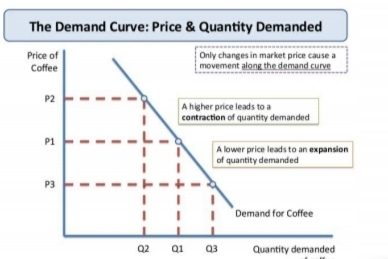
Law of Demand
The law of demand was given by Alfred Marshall. It is a partial equilibrium analysis and
states that there is an inverse relationship between price of the commodity and the quantity
demanded of it.
Demand Curve: It is the graphical presentation of the law of demand
Demand Schedule: It is the tabular presentation of the law of demand.
Market Demand: It is the horizontal summation of individual demands. It is affected by the
population levels. Market demand curve is flatter as compared to the individual demand.
Reasons for downward sloping demand curve
1. Law of Diminishing Marginal Utility: This states that the marginal
utility of a good or service declines as its available supply increases.
2. Income effect: The change in consumer’s purchases of the goods as a
result of a change in their money income
3. Substitution effect: Effect of a change in the relative prices of goods
on consumption pattern
4. Different uses of a commodity
5. Size of the market
Exceptions to the Law of Demand
1. Veblen Effect: Goods having prestige value. Veblen
propounded the doctrine of conspicuous consumption. Higher
the price of the commodity, more will be the prestige derived
from it
2. Giffen goods: The demand curve for a giffen goods is an
upward sloping curve
3. Ignorance
4. Expectations
5. War
Bandwagon Effect: It arises because individuals demand
commodities because others are doing so, or in simple words, it is in
fashion.
Snob Effect: It arises due to the desire to purchase a commodity
having prestige value so as to look different or exclusive than others.
CHANGES IN DEMAND
Increase or Decrease in Demand
• Leads to shift in the demand curve.
• Caused by Shift Factors of Demand (Factors other than price)

Expansion or Contraction of Demand
• Leads to movement in the demand curve.
• Caused due to price.
Demand for Durable goods
• Durable goods can be stored, hence the prices
are not volatile.
• Consumption can be postponed.
Derived Demand
It is the demand for goods which are used to produce other goods. Example Labour.
ELASTICITY OF DEMAND
The concept of elasticity of demand was given by Marshall.
Elasticity of demand measures the responsiveness or change in
demand due to factors like price, income, price of related goods,
etc.
Price elasticity : Price elasticity is the proportionate change in
quantity demanded divided by the proportionate change in price.
Degrees of Price Elasticity:
Unitary Elastic e=1
Elastic e>1
Inelastic e<1
Perfectly Elastic e=Infinity
Perfectly Inelastic e=0
Measurement of Price Elasticity of Demand
a. Proportionate or Percentage Method: Here, the price elasticity is
measured by its coefficient Ep. This measures the percentage change
in the quantity of a commodity demanded resulting from a given
percentage change in its price.
b. Point Elasticity Method = 𝑳𝒐𝒘𝒆𝒓 𝑺𝒆𝒈𝒎𝒆𝒏𝒕 /𝑼𝒑𝒑𝒆𝒓 𝑺𝒆𝒈𝒎𝒆𝒏𝒕

c. Arc Elasticity Method: It is used when price and quantity
changes are somewhat large. It is the measure of the average
responsiveness to price change exhibited by a demand curve over
some finite stretch of the curve
d. Total Expenditure Method: Evolved by Marshall. By comparing
the total expenditure of a purchaser both before and after the
change in price, it can be known whether their demand for a good
is elastic, unity or inelastic.
e. Revenue Method: Elasticity will be measure in this method using
the concepts of AR and MR. e= AR/(AR-MR)
Income Elasticity: It is the responsiveness of change in quantity
demanded due to change in income levels.
Normal Good (ey) > 0
Inferior goods (ey) < 0
Luxuries (ey) > 1
Necessities 0 < ey < 1
Engel curve: Engel curve is the graphical presentation of relationship
between income and quantity demanded.
Necessities (+ve relation)
Luxuries (+ve relation)
Inferior goods (+ve relation)
Cross Elasticity of Demand measures the degree of responsiveness
of change in the demand for one good in response to the change in
price of another good.
Ec = 𝐏𝐫𝐨𝐩𝐨𝐫𝐭𝐢𝐨𝐧𝐚𝐭𝐞 𝐜𝐡𝐚𝐧𝐠𝐞 𝐢𝐧 𝐭𝐡𝐞 𝐪𝐮𝐚𝐧𝐭𝐢𝐭𝐲 𝐝𝐞𝐦𝐚𝐧𝐝𝐞𝐝 𝐨𝐟 𝐗 /
𝐏𝐫𝐨𝐩𝐨𝐫𝐭𝐢𝐨𝐧𝐚𝐭𝐞 𝐜𝐡𝐚𝐧𝐠𝐞 𝐢𝐧 𝐭𝐡𝐞 𝐩𝐫𝐢𝐜𝐞 𝐨𝐟 𝐠𝐨𝐨𝐝 𝐘
Goods Cross Elasticity
1. Substitutes Positive
2. Complements Negative
3. Unrelated Zero
QUESTIONS FOR CLARITY
1. The value of the best alternative forgone when a decision is made defines
(A) economic good.
(B) opportunity cost.
(C) scarcity.
(D) trade-off.
2. Which of the following problems do all economic systems face?
I. How to allocate scarce resources among unlimited wants
II. How to distribute income equally among all the citizens
III. How to decentralize markets
IV. How to decide what to produce, how to produce and for whom to produce
(A) I only
(B) I and IV only
(C) II and III only
(D) I, II and III only
3. A downward sloping demand curve can be explained by
I. diminishing marginal utility. II. diminishing marginal returns.
III. the substitution effect. IV. the income effect.
(A) I only
(B) I and III only
(C) I and IV only
(D) I, III and IV only
4. Which of the following will not change the demand for oranges?
(A) A change in consumer’s incomes
(B) A change in the price of oranges
(C)A change in consumer’s taste for oranges
(D) All the above changes the demand for oranges
5. If hot dogs are an inferior good, an increase in income will result in
(A) An increase in the quantity demanded for hot dogs.
(B) A decrease in the quantity demanded for hot dogs.
(C) No change in the quantity demanded for hot dogs.
(D) None if the above
Answers :
1) B 2) B 3) D 4) D 5) B
THEORIES OF DEMAND
1. Cardinal or Marshallian Analysis
Cardinal school is the oldest school in case of theories of demand.
Concept of Utility was originally given by Bentham, however, it was formally
introduced by Jevons. He defined utility as the power of a commodity or service to
satisfy human wants.
Assumptions of cardinal analysis are as follows:
a. Utility can be measured.
b. Consumer is rational
c. Money is a measuring mode of utility.
d. Marginal utility of money is constant: The concept of Marginal Utility of money was
given by Daniel Bernoulli.
e. Utilities are additive in nature.
f. Utilities are independent.
g. It is based on introspection.
Theories under Marshallian Analysis
a. Law of Diminishing Marginal Utility: It is also known as Gossen's First law.
Law of Diminishing Marginal Utility states that as the consumer consumes more and
more of a commodity, the marginal utility derived on consuming each additional unit
keeps on declining.
Total Utility (TU): Total utility is the total satisfaction achieved after consuming all the
units of a particular commodity.
Marginal Utility (MU): Marginal Utility is the additional or incremental utility achieved
after consuming additional unit of a commodity.
“Marginal Utility curve is simply the slope of the total utility curve”.
Marginal Utility explains the relationship between demand and price.
It explains the paradox of value. Marginal utility determines the price of a commodity
and not the total utility.
b. Law of Equi-Marginal Utility: It is also known as Gossen’s Second Law. The law
states that the marginal utility derived should be equal to that derived from the last
rupee spent.
The law is more associated with the consumer’s equilibrium. Consumer will reach the
equilibrium point when:-
• In case of single good: MUx = Px
• In case of several goods: MUm = (MUx/Px) = MUy/Py = ……
2. Ordinal or Hicksian Analysis : Utilities cannot be measured.
Assumptions of the theory:
a. Utilities can be ranked.
b. Consumer is rational.
c. Indifference curve is based on weak ordering, that is, it considers both preferences and
indifference.
d. The consumption follows a transitive pattern.
e. Continuity: The consumption follows a smooth continuous curve which can be drawn.
f. Diminishing Marginal Rate of Substitution: MRSXY = ΔY/ΔX = MUx / MUY
Note: MRSXY is also the slope of Indifference curves.
Indifference curves
The convex shape of IC shows
diminishing MRS.
Indifference Map: Set of ICs
Why the MRS is decreasing?
• Want of the good is satiable.
• Goods are imperfect substitutes of
each other.
Shapes of Indifference Curves are:
Perfect Substitutes: Straight line
Perfect Compliments: L Shaped

Budget Line(Price Line)
When there is a change in income levels, it leads to shift in the budget line. When there is
a change in prices, it will lead to the movement in the budget line.
Consumer Equilibrium
It is the point of tangency between Indifference curve and budget line
MRSXY = MUX / MUY = (-) PX / PY
Conditions for consumer equilibrium
First Order Condition: MRSXY = MUX / MUY = (-) PX / PY
Income Effect
To trace the income effect, we have an Income Consumption curve which shows the changes in
consumer equilibrium with changes in income.
Note:- Normal goods are those whose consumption increases with increase in income, while
inferior goods are those whose consumption decreases due to increase in income.
Substitution Effect
Substitution effect traces the changes in consumption of commodities when the relative prices
change.
In case of tracing the substitution effect, we keep the real income as constant so that we can
know the relative change in the prices
Price Effect
Price effect is the change in demand due to change in the price of the commodity, other things
remaining the same. To trace the changes in price effect, we have price consumption curve.
Price Effect = Income Effect + Substitution Effect
Hints for Decomposition of Price Effect into Income Effect and Substitution Effect:-
Goods Price Effect Income Effect Sub. Effect
1. Normal Negative Positive Negative
2. Inferior Negative (I.E.<S.E.) Negative Negative
3. Giffen Positive (I.E. > S.E.) Negative Negative
3. Revealed Preference Theory: The theory was given by Samuelson in 1938. It is a form
of ordinal ranking and is based on the concept of strong ordering. The theory is behavior
based and the choice of the consumer reveals the preference.
Assumptions of the theory are:
a. Consistency
b. Transitivity
c. Choice is always made
d. Income will be fully spent.
e. More is preferred to less.
Indirect Revealed Preference
In this case more than two goods are involved. For example, if A is preferred to B, and B is
preferred to C, then A is indirectly preferred to C.
Indifference curve uses real income for estimating the level of satisfaction whereas revealed
preference theory uses real income for estimating the purchasing power
Fundamental Theorem of Consumption
The theorem was given by Samuelson. It states that price and quantity will be negatively
related if we have positive income effect of demand.
In case of indifference curve analysis, real income is used in the sense of level of satisfaction.
In case of revealed preference, real income is used in the sense of purchasing power.
4. Hicks’ Logical Ordering
This theory is the revised version of Hicks’ own theory in his work “A Revision of
Demand Theory” in 1956. He was influenced by Samuelson’s work and hence used
econometrics in his theory, keeping the original assumption that utility is ordinal in nature.
5. Consumer Behaviour Under Uncertainty
The theory was propounded by Neumann and Morgenstern and is commonly known as
N-M
Utility Index. They have considered the role of both risk and uncertainty.
Expected utility of a lottery can be calculated using the weighted sum of the utilities
associated with the outcomes with probabilities acting as weights.
E(U(L)) = P1 (U(A)) + (1-P1)(U(B))
For a risk averse person, U[E(L)] is greater than E[U(L)] and marginal utility of money is
falling.
For a risk lover, U[E(L)] is less than E[U(L)] and marginal utility of money is rising.
For a risk neutral person, U[E(L)] is equal to E[U(L)] and marginal utility for money is
constant through all income levels.
Risk premium is to protect the risk averse person to avoid risk.
Two measures of risk aversion were given by Arrow and Pratt.
a. Absolute measure: It is measured using the formula:
[-U’’(W)/U’(W)]
where, W is a measure of wealth
[-U’’(W)/U’(W)] is positive Risk Averse
[-U’’(W)/U’(W)] is negative Risk Lover
[-U’’(W)/U’(W)] is zero Risk Neutral
b. Relative measure: It helps in comparing the attitude of workers towards risk and is
measured using the formula
W*RA
Where, RA is the relative attitude towards risk.
Bernoulli’s hypothesis: The theory assumes that majority of the population is risk averse
and hence marginal utility of money is declining. For the risk averse person, the effect of
gain received from the lottery will be less than the effect of loss incurred and hence he
will never choose a 50- 50 probability.
Friedman-Savage Hypothesis: According to this theory, the marginal utility will not be
constant over the entire range, that is, it will both increase and decrease. The attitude of
the consumer would depend on whether the marginal utility of money is increasing or
decreasing.
Markowitz Theory: According to his theory, there can be both risk lovers as well as risk
averse individuals. The marginal utility of money will not be constant over the entire
range. However, in his theory, small increases or decreases in income will increase the
marginal utility of money but large changes in income will always lead to decrease in
marginal utility of money.
St. Petersburg Lottery/Paradox: The paradox states that when the number of participants
are less, then this might lead to infinite expected value. In the case, an individual will always
accept the lottery.
Investor Choice Problem : Budget constraint will be an upward sloping line because there
is a positive trade-off between risk and return.

QUESTIONS FOR CLARIFICATION
1. Which of the following is an example of a normative statement?
(a) Since this good is bad for you, you should not consume it.
(b) This good is bad for you.
(c) If you consume this good, you will get sick.
(d) People usually get sick after consuming this good.
2. Suppose the demand curve for a good shifts rightward, causing the equilibrium price to
increase. This increase in the price of the good results in
(a) a rightward shift of the supply curve.
(b) an increase in quantity supplied.
(c) a leftward shift of the supply curve.
(d) a leftward movement along the supply curve.
3. Equilibrium is defined as a situation in which
(a) neither buyers nor sellers want to change their behavior.
(b) no government regulations exist.
(c) demand curves are perfectly horizontal.
(d) suppliers will supply any amount that buyers wish to buy.
4. The change in price that results from a leftward shift of the supply curve will be greater if
(a) the demand curve is relatively flat than if the demand curve is relatively steep.
(b) ) the demand curve is relatively steep than if the demand curve is relatively flat.
(c) the demand curve is horizontal than if the demand curve is vertical.
(d) the demand curve is horizontal than if the demand curve is downward sloping.
5. If the price elasticity of demand for a good is less than one in absolute terms, we say
consumers of this good
(a) are not very sensitive to price.
(b) are not very sensitive to the quantity they demand.
(c) are very sensitive to price.
(d) are elastic.
Answers:-
1) A 2) B 3) A 4) B 5) A
PRODUCTION THEORY
A production function shows the technical relationship between the inputs and outputs.
Q=f(L,K)
Assumptions of production function are:
1. State of technology is assumed to be constant.
2. Production function is with reference to a particular period of time.
Production function
1 factor variable, others fixed
(Law of variable prop. because proportion varies, SR law)
All factors variable
(Returns to scale of inputs, LR Law)
Law of Variable Proportions/Returns to a Factor
It is a short run theory in which there is atleast one factor which is fixed, that is, it cannot change.
Thus, this law deals with the changes in the factor proportions.
Beyond a certain point, the MP of the factor would diminish.
Assumptions :- (1) Tech is fixed and constant
(2) Some inputs should be ript constant
(3) Various factors can be combined to produce
Stages of Law of Variable Proportions
Stage 1: Increasing returns to a factor
Under this stage the marginal product increases, reaches maximum and starts decreasing. The
stage ends
where the average product reaches maximum.
In this stage MP of the fixed factor is negative.
Stage 2: Diminishing returns to a factor
Under this stage, the marginal product decreases, average product starts falling. The stage ends
when
marginal product reaches zero.
Stage 3: Negative Returns to a Factor
Under this stage, the marginal product of the variable factor becomes negative as a result of
which the total product starts falling.
NB:- A point to remember here is that in stage 1, the marginal product of fixed factor is negative
because it is in excess of the variable factor. On the other hand, in stage 3, the marginal product
of a variable factor is negative because it is in excess of the fixed factor.
Isoquants/Equal Product Curves/Iso-Product Curves
Isoquants is the locus of various combinations of input producing the same level of output.
MRTS Slope of isoquants
• No of units of capital gives up to get me unit of labour, output to be the same.
• Diminishing is nature (Convexity)
If isoquant is concave linear, the optimum production would be at a corner solution
Elasticity of Substitution
1. Perfect substitutes: Marginal Rate of technical substitution is constant and elasticity of
substitution is equal to infinity.
2. Perfect Complements: Marginal rate of technical substitution is zero and elasticity of
substitution is also equal to zero.
Types of Production Functions
1. Linearly Homogenous Production Function
Q = f(L,K)
If we multiply the production function with a constant say m, Q = f(mL, mK)
Taking m to be common, we get; Q = m.f(L,K)
Q= m.Q
Anything raise to the power m, gives us the degree of homogeneity.
2. Cobb-Douglous Production Function
It was given in 1928 and is represented as follows:
Q = ALαKβ
Where:
Q = Output level, A = State of Technology, L = Labour, K = Capital, α = Share of Labour in
production, β = Share of capital in production
The features of C-D production function are:
• Linearly Homogenous Production Function
• Constant Returns to Scale
• Elasticity of Substitution is equal to one
• α tells the output or production elasticity of labour, β tells the output or production elasticity of
capital and they both are constant.
α + β = 1 Constant Returns to Scale
α + β > 1 Increasing Returns to Scale
α + β < 1 Decreasing Returns to Scale
Euler’s Theorem: If the factors are paid on the basis of their marginal productivity, then
ultimately the total output will be exhausted. It holds true in linearly homogenous production
function.
MPL * L + MPK * K = Q
3. CES Production Function
It was given in 1961 by Arrow, Minhas, Chenery and Solow
Q = Ɣ[ϨL-ϱ + (1-Ϩ)K-ϱ] -1/ ϱ
Where
Ɣ = Coefficient of technical efficiency; Ɣ > 0
Ϩ = Distribution Parameter; 0 < Ϩ < 1
ϱ = Substitution parameter
Elasticity of Substitution = 𝟏 /(𝟏+𝛠)
Ridge Lines: Ridge lines are the locus of points where marginal productivity of atleast one factor
is zero.
Isoclines: Isoclines is the locus of points in which marginal productivity of inputs is kept constant.
There are two ridge lines A and B. At A, the marginal
productivity of capital is zero and points above A
show negative marginal productivity of capital.
At B, the marginal productivity of B is Zero and is
negative at all points below it.
The optimum stage of production is the region between the two ridge lines and hence is
called the region of economic production.


Returns to Scale
It is a long run law in which all the factors are variable in nature and factor proportions do not
change. All inputs will be varied by the same proportion.
Stages of Returns to Scale
1. Constant Returns to Scale: Under this, the change in proportion of inputs is equal to the
change in proportion of outputs. Isoquants are equi-distant
2. Decreasing Returns to Scale: Under this, the change in proportion of inputs is greater than the
proportionate change in outputs. The distance between the isoquants keep increasing.
3. Increasing Returns to Scale: Under this, the change in proportion of inputs is less than the
change in proportion in outputs. The distance between the isoquants would keep decreasing.
Economies of Scale
• Reasons for Increasing, Decreasing or Constant Returns to Scale are explained by the
Economies of Scale.
Internal Economies of Scale Firm Based
External Economies of Scale Industry Based
Real Economies: Real economies are experienced when we reduce the quantity purchased of our
physical inputs.
Pecuniary Economies: Pecuniary economies are experienced when we purchase large quantities
of physical inputs so that the overall price paid is less. For example, wholesale prices.
Relationship between Returns to Scale and Returns to a factor
Returns to Scale When Capital is held constant
Constant Returns to scale Returns to a factor say MPL will diminish when capital is
held constant.
Decreasing Returns to scale Returns to a factor MPL will diminish at a rapid pace.
Increasing Returns to scale There can be two possibilities:
1. If there are strong increasing returns to scale then
returns to a factor MPL will increase.
2. If there is a slight increasing returns to a scale then
returns to a factor MPL will decrease.
Single Product Firm
For a firm producing single output, equilibrium will occur at the point of tangency of
isoquant and the iso- revenue line
Multi-product Firm
Production Possibility Frontier: It is the combination of two goods which can be produced
given the technology or level of resources.
Iso-Revenue line: It is the locus of points of combination of two goods produced which generate
equal revenue.
Slope of PPC is the Marginal Rate of Product Transformation (MRPT) which is increasing
because different resources are suited to produce different goods.
MRPTXY = 𝐌𝐂𝐱 / 𝐌𝐂𝐲
Equilibrium point will occur where MRPTXY = 𝐌𝐂𝐱 / MCy= 𝐏x / 𝐏𝐲
Expansion Path: It is the locus of point of revenue maximisation. It is also known as scale line
because it tells how firms change their scale of production.
Price Effect
In case of production theory, the price effect is the sum of output effect and substitution
effect.
In case when factors of production are substitutable, then substitution effect is greater than the
output effect implying that, if price of labor decreases, then labor would be used more as
compared to the other input.
In case the goods are complementary, then output effect is more than the substitution effect
implying that with decrease in price of labor, more of both factors will be used.
Technical Efficiency: It implies maximizing the output with given inputs.
Economic Efficiency: It implies minimizing the cost to produce a given level of input.
Theory of Cost
In short run, we assume one factor of production to be variable and rest all are fixed.
In the long run, we assume technology and prices to be constant.
Shift Factors: These are the factors shifting the cost function other than the output.
In the long run, technology and prices are the shift factors
In the short run, the fixed factors are considered to be the shift factors.
Types of Cost
1. Explicit Cost: It is also known as the accounting cost, private opportunity cost. These costs are
out of the firm or cost of hiring a factor of production.
2. Implicit Cost: Also known as the imputed cost. These are the prices of owned services and are
included in the average cost.
3. Economic Cost: It is the sum of explicit and implicit cost.
4. Opportunity Cost: It is the cost of next best alternative and is a part of implicit cost. It is also
known as transfer earnings.
5. Historical Cost: It is the original price of the factor of production when bought in the past. It is
irrelevant in the production process.
6. Sunk Cost: It is a kind of historical cost which cannot be recovered. Even sunk costs are not
relevant to decision making.
Economic Profits = Total Revenue = Economic Costs
Total Cost = Total Fixed Cost + Total Variable cost
Average Cost = Average Fixed Cost + Average Variable Cost
Marginal cost is the change in Total cost due to the change in inputs used for production
Relationship between Average Cost and Marginal Cost
When AC is falling, marginal cost is falling more than AC. When AC is minimum, AC = MC
When AC is rising, MC rises more than AC
Long Run Costs
Long Run Costs are less than or equal to short run costs, and are hence flatter as compared to the
short run costs.
Long Run Average cost curve is also known as the planning curve. Plants are used at less than
full capacity at point left to the minimum point and are used at more than full capacity at points
right to the minimum point. The optimum plant size is when it operates at minimum LAC.
Recent Developments in the Cost Theory
1. Saucer Shaped LAC
The shape is such due to the reserve capacity
Reserve Capacity: Saucer shaped Cost curve is due to the existence of reserve capacity of the
firm. This portion indicates a horizontal portion in the average cost curves.
2. L-Shaped or continuously falling LAC curve
The reasons for continuously falling LAC curve are:
a. Economies of Scale b. Technological Progress
3. Learning Curve: This was given by Kenneth Arrow.
It includes the concept of learning by doing. It states that the increase in cumulative output leads
to decline in per unit cost due to learning by doing.
Economies of Scope: Joint production of a good is more efficient than the separate production
by two firms producing the same good.
Diseconomies of Scope: Joint production is less than the individual production.
QUESTIONS FOR CLARITY
1. An isoquant curve shows
a. all the alternative combinations of two inputs that yield the same maximum total product.
b. all the alternative combinations of two products that can be produced by using a given set of
inputs fully and in the best possible way.
c. all the alternative combinations of two products among which a producer is indifferent because
they yield the same profit.
d. both (b) and (c).
The Marginal rate of technical substitution is
2. the rate at which a producer is able to exchange, without affecting the quantity of output
produced, a little bit of one input for a little bit of another input.
b. the rate at which a producer is able to exchange, without affecting the total cost of inputs, a
little bit of one input for a little bit of another input.
c. the rate at which a producer is able to exchange, without affecting the total inputs used, a little
bit of one output for a little bit of another output.
d. a measure of the ease or difficulty with which a producer can substitute one technique of
production for another
3. For a given short-run production function,
a. technology is assumed to change as capital stock changes.
b. technology is assumed to change as the labor input changes.
c. technology is considered to be constant for a given production function relationship.
d. technology is assumed to change positively until diminishing returns set in and then it changes
in the other direction.
4. A tangency point between an isoquant and an isocost line identifies
a. the least costly combination of inputs required to produce various levels of outputs.
b. the various levels of output that can be produced using a given level of inputs.
c. the various combinations of inputs that can be used to produce a given level of output.
d. the least costly combination of inputs required to produce a given level of output.
5. If a profit-maximizing firm’s marginal product of labor equals 1 ton of output, while the
marginal product of
capital equals 7 tons of output and the use of capital is priced at $14 per unit, then
a. the price of labor must be $2.
b. the price of labor must be $7.
c. the price of labor must be $14 as well.
d. none of the above is true.
6. Which of the following statements about marginal cost is incorrect?
a. A U-shaped marginal cost curve implies the existence of diminishing returns over all ranges of
output.
b. When marginal cost equals average cost, average cost is at its minimum.
c. In the short run, the shape of the marginal cost curve is due to the law of diminishing marginal
returns.
d. When marginal cost is falling, total cost is rising.
7. Which of the following statements about the relationship between marginal cost and average
cost is correct?
a. When MC is falling, AC is falling.
b. AC equals MC and MC’s lowest point.
c. When MC exceeds AC, AC must be rising.
d. When AC exceeds MC, MC must be rising.
Answers:-
1)A 2)A 3)C 4)D 5)A 6)A 7)C
MARKET STRUCTURES
Types of Markets:- 1. Perfect Competition
2. Monopoly
3. Oligopoly
4. Monopolistic Competition
1. Perfect Competition
Features of perfect competition are:
a. Large number of buyers and sellers. b. Free entry and exit. c. Perfect information.
d. No transport cost. e. Homogenous Product
Perfect Competition vs Pure Competition
Perfect competition is a wider concept and is perfect in all contexts. On the other hand, pure
competition is a narrower concept in which there is freedom from monopoly errors and freedom
from entry and exit.
Time element
Marshall gave the concept and he divided time on the basis of response of supply
(1) Market period /very short time period – supply fixed and there are no adjustments
(2) Short period – Expand output with given equipment No change in plants or given capital.
(3) Long period – New entry and exit, New plants/abandon old ones, Full adjustment of all factors
and all costs.
Under Perfect Competition, MR = AR = Price
Short Run Equilibrium
Two conditions need to be satisfied for attaining the equilibrium level:
1. Marginal Cost (MC) = Marginal Revenue (MR)
2. MC should cut MR from below
• In the Short run, there are 3 possibilities
1. Super Normal Profits 2. Normal Profits 3. Losses


Long run
In the long run, a perfectly competitive industry earns only normal profits, that is,
Price = AR = MR = LMC = LAC = SAC = SMC
Important:-
❑ A perfectly competitive firm does not quit the industry even if it incurs losses in the short run
because they can’t alter the fixed capital equipment in the short run. As a result, they will have
to incur the losses equal to fixed cost even when they shut down. Thus, they continue
production in the short run even when they incur losses.
❑ A perfectly competitive firm is in business even when economic profits are zero because
economic profits include the opportunity costs. So at zero economic profits, firms still earn a
return on capital invested. So at zero economic profits, the firms still earn a return on the
capital invested.
Consumer surplus :- Price consumers are
willing to pay- what they actually pay
Producer’s surplus :- Mkt price at which
sellers sell min price they are willing to sell.
❑ This diagram explains the consumer
surplus and producer surplus explained
by Marshall
❑ Hicks also analyzed the Consumers
Surplus based on indifference curve analysis

2. Monopoly
Features:
a. Single seller b. No close substitutes c. Barriers to prohibit the entry of new firms.
d. Affects no other seller by its own action. e. Firm and industry are one single entity.
f. The demand curve in case of a monopolist is a downward sloping curve.
Pure Monopoly
Single Seller, no substitutes, cross elasticity = 0, price elasticity = 1. Thus Total revenue remains
constant
Natural Monopoly
Single Seller, the good produced has substitutes, cross elasticity is low.
Legal/Statutory Monopoly: The government provides the legal status through patents or
copyrights.
Price and Marginal Cost under Monopoly
Price difference from MC = f (Price elasticity
at that point on AR curve) Smaller the
elasticity, greater the difference between
price and MC. Therefore,
Monopoly price = f (MC, Price elasticity)
Where, Monopoly price and MC are
positively related, and Price elasticity
and Monopoly price are negatively related.
Monopoly Equilibrium And price Elasticity of Demand
Monopolist will never be in when ep < 1 We know,
MR = AR [(e-1)/e]
So when e < 1, MR becomes negative, implying a fall in total revenue. So it will not be rational for
the monopolist to operate at a point where Marginal revenue is negative.

NB: When the marginal cost is zero, monopolist operates at the point
where price elasticity of demand is equal to one.
❑ Average revenue is decreasing because more can be sold at lower price. MR is below AR
because its fall is twice the fall of AR. Therefore, Price is more than marginal cost.
❑ Cost curves remain the same.
❑ There is no supply curve in monopoly. No unique price-quantity relationship
Short Run:
Conditions of equilibrium
1. MR = MC
2. MC should cut MR curve from below
In short run, a monopolist can earn super-normal profits, normal profits or can even incur losses.


Long Run: In the long run, a monopolist earns only super normal profits because there are no
barriers to entry.
Conditions for equilibrium:
a. Short run Average cost = Long run Average Cost (LAC)
b. Marginal Revenue = Long Run Marginal Cost = Short run Marginal Cost
c. Price > LAC
Monopoly regulation
a. Price regulation:- 1. MC Pricing (Price is charged equivalent to the MC)
2. AC Pricing (Price is charged equivalent to AC)
b. Taxes: Specific Tax (It will affect both MC and AC. If specific tax increases, price
increases and entire burden fallson the consumers. It is not a good way
to regulate a monopoly. )
Lump Sum Tax(It only affects on AC. Only profits would be reduced and
there is no change in quantity and price)
Price Discrimination: Price discrimination is an act of charging different prices from different
consumers for the same good.
Degrees of price discrimination
1. First Degree of Price Discrimination: Marginal Revenue curve also becomes the
demand curve, Marginal Revenue = Price, Each consumer is charged his respective reservation
price, It is also the ‘Take it or leave it’ strategy.
2. Second Degree of Price Discrimination: It is applicable to a particular section of
goods, Goods can be divided into different parts, Goods included are either recorded or billed or
metered.
3. Third Degree of Price Discrimination: • It is possible when the elasticities between
the two markets are different.
Inter temporal price discrimination
Separating customers with different demand functions into different groups which leads to
charging diff. prices at different points of time.
Peak load pricing:- Charge high prices at peak times because capacity constrain to cause MC to
be high
Two part tariff:- Consumers are charged both entry of usage fees.
Degree of Monopoly Power: The monopoly power determines the extent to which a monopolist
has control over either prices or quantities.
Measures of Monopoly Power:
1. Performance based: It is an outcome of the use of the monopolists’ ability.
❑ Elasticity of Demand: Monopoly power is the inverse of elasticity of demand.
MP= 1/Ed
❑ Lerner’s Measure: P − MC /P or P − MR/P or 1/Ed
❖ Greater the difference between price and marginal cost, greater will be the Lerner's
measure and thus greater will be the monopoly power.
❑ Cross Elasticity of demand: The measure was given by R.Triffin and thus it is also known as
Triffin’s Measure. Monopoly power is determined by how many substitutes does the good
has. More the number of substitutes, less will be the monopoly power. Therefore, monopoly
power is measured by taking the inverse of cross elasticity of demand.
Monopoly Power = 1 /ec
❑ Bain’s rate of return: P − LAC P
Higher the difference between price and average cost; higher will be the monopoly power.
2. Structural Based Measures:
❑ Concentration Ratio (CR): It measures the extent to which the large firms control the output.
❑ Hirfindahl-Hirschman Index (HHI) = ⅀x ^2
where x is the share of each firm.
xi = Xi / Total Industry size
❑ Gini Coefficient: It is a measure of inequality in a distribution and is measured with the help of
Lorenz curve.
Gini coefficient = 1 (In case of Monopoly)
= 0 (In case of Perfect Competition)
3. Monopolistic Competition:
Joan Robinson: "The Economics of Imperfect Competition"
E.H. Chamberlin: "The Theory of Monopolistic Competition"
Features of monopolistic competition are:
a. Large number of buyers and sellers b. Non-price competition c. Selling cost
d. Some influence over the price e. Non-price competition
f. Product variation
Perceived demand curve: It is subjective in nature. If one firm is changing prices, other firms
keep their price constant; it would cause a relative change in prices making the perceived demand
curve slide down.
Proportionate demand curve: If number of firms increase, the curve shifts leftwards implying
that the proportionate quantity demanded of that firm’s output decreases.
❑ In case of monopolistic competition, a firm can earn super normal profits or normal profits or
even losses in the short run; while in the long run it earns only normal profits.
The conditions of equilibrium are:
a. MC = MR
b. MC should be rising
Chamberlin explained the concept of Excess capacity in terms of perceived and
proportionate demand curve.
In the long run, the perceived demand curve shifts
down due to active price competition.
Excess Capacity: Extent to which the long run
output is falling short of ideal output is called
excess capacity. It must be noted that excess
capacity is a long run concept and is not applicable
in the short run.

❑ There is always an excess capacity in case of monopolistic competition due to downward
sloping demand curve. Greater the elasticity of demand curve, lesser will be the excess
capacity.
Causes of excess capacity
1) Downward sloping dd curve
2) Product differentiation
3) Entry of a very large no. of firms
Cassel’s View on excess capacity: According to him, excess capacity can be divided into two
parts: Firstly, Individual optimum, Secondly, Social Optimum.
Chamberlin’s View on excess capacity: According to him, excess capacity will arise when firstly,
there is free entry and secondly, when there is no price competition.
Price Output Equilibrium under Monopolistic Competition and Perfect Competition:
1) Price is greater than MC under Monopolistic Competition.
2) Long run equilibrium under Monopolistic Competition is established at less than technically
efficient scale.
No profits or normal profits by both Monopolistic Competition and Perfect Competition.
Moreover, output is less in monopolistic competition as compared to perfect competition.
3) Price under Monopolistic Competition is greater than competitive price.
Monopolistic Competition & Economic Efficiency.
Economic inefficiency is caused by two factors:
1. P > MC: Value to > MC of \ producing customers
2. Excess capacity

1. A firm operating in a perfect market maximizes its profit by adjusting
a. its output price until it exceeds average total cost as much as possible.
b. its output price until it exceeds marginal cost as much as possible.
c. its output until its marginal cost equals output price.
d. its output until its average total cost is minimized.
2. In the short run, no firm operates with a loss, unless
a. variable cost equals fixed cost.
b. variable cost falls short of fixed cost.
c. total revenue covers variable costs.
d. total revenue covers fixed cost.
3. In perfect competition, when economic profits exist in the short run, they are very tenuous
because
a. costs will inevitably increase and eliminate profit.
b. price will fall because market supply will increase.
c. firms are driven to increase output in the short run to the point where average total cost will
equal price.
d. firms are driven in the short run to reduce output until average total cost equals price.
4. If a firm is producing where its SMC = price and the LMC is less that LAC, then it would do
better in the long run by
a. increasing output with its existing plant until LMC equals price.
b. increasing plant size until LMC and SMC are identical and equal to price.
c. decreasing plant size until LAC, SAC, and price are equal.
d. doing nothing because it is already at the long-run profit maximizing point.
5. In the long run, a profit-maximizing monopoly produces an output volume that
a. equates long-run marginal cost with marginal revenue.
b. equates long-run average total cost with average revenue.
c. assures permanent positive profit.
d. is correctly described by both (a) and (c).
Suppose that an excise tax is imposed on the monopolist’s product. If the monopolist’s marginal
cost is
6. horizontal in the relevant range, which of the following statements must be true?
a. The price will increase by an amount less than the tax.
b. The price will increase by an amount equal to the tax.
c. The price will increase by an amount greater than the tax.
d. An excise tax will have no effect on the price-output decision of a monopolist.
7. Since entry is barred in a monopoly, in the long run the monopolist will
a. do nothing since entry will not force an adjustment.
b. adjust output but leave the price at the short run profit maximizing level.
c. adjust price but leave the output at the short run profit maximizing level.
d. adjust both price and output levels to reflect long run scale of plant adjustments.
8. A monopolistically competitive market is characterized by all of the following except
a. easy entry.
b. differentiated products.
c. excess capacity.
d. economic profit in the long run.
9. A monopolistically competitive firm differs from a perfectly competitive firm in that, unlike the
perfectly
competitive firm, it
a. faces a downward sloping demand curve.
b. can change the characteristics of its product.
c. can vary the price of its product.
d. tends to operate with excess capacity.
e. all of the above.
Answers:-
1) C 2) C 3) B 4) B 5) A 6) A 7)D 8)D 9)E
Oligopoly:
Pure oligopoly (Without product differentiation; Homogenous)
Differentiated Oligopoly (With product differentiation; close substitutes)
Features of Oligopoly are:
a. Few Sellers b. Same good/different goods c. Interdependence
d. Selling costs e. Group behaviour f. Indeterminate demand curve
Causes for existence of oligopolies.
1) Economies of scale :- When economies of scale are strong, Market may be too small to
support large no. of firms.
2) Barriers to entry:- It include both Technological and legal barriers to entry
3) Product Differentiation: This gives the firms some kind of Market Power
4) Firm-created causes of oligopolies
a) Merging
b) Predatory Pricing :- Lowering the price so much to drive the rivals out of the market.
Collusive Oligopoly: Firms recognized that they can help each other in the form of:
a. Cartel: Group of firms mutually decide price and quantity and get rid of the uncertainty.
Types of cartel:
Perfect Cartel (Members cannot cheat. One firm out of the group decides the price and output
for all. The cartel acts as a multi-plant monopolist. It is a tight cartel because one firm has all the
control. The objective is joint profit maximisation.
Market sharing cartel (These are loose cartels which share the market)
Price leadership: Under this, one firm will set its price which will be followed by other
firms.
Low cost firm (Set a low price which is to be followed by high cost firms)
Dominant price leadership (Firm with maximum market share leads)
Barometric Price leadership (Firm which is oldest and most experienced)
Exploitative or Aggressive Price Leadership: (Large or dominant firm follows aggressive price
policies, threatens other firms)
Non-collusive oligopoly
Nash Equilibrium, given by John Nash 1951. It implies a set of strategies or action in which each
firm does the best it can, given its competitors.
a. Cournot Model: The model was developed in 1838 by Augustin Cournot.
Assumptions are:
• There are two firms.
• Firms produce homogenous goods.
• Firm assumes that other firm will keep its output constant.
• Marginal cost of producing a good is zero.
• The firms simultaneously take the decision.
The output produced by other firm is the ½ of the remainder. In the end, both firms produce
1/3rd of the total output.
If there are more than two firms, then total output produced in the market would be n/(n+1)
where n is the number of firms in the market. Suppose there are 10 firms, then total output
produced would be 10/11 of the perfectly competitive output and each firm will produce 1/11 of
the output.
• Cournot price is between monopoly price and competitive price. Mp > Cp > P.C.p
• Cournot price is the 2/3rd of the most profitable price.
• Cournot output is the 2/3rd of the maximum output or perfectly competitive output.
b. Bertrand Model: The model was developed in 1883.
• It works on the assumption that other firm will keep the price constant.
• Firms have an unlimited productive capacity to meet the demand requirements.
• The model is based on the price cutting behaviour.
• By under-cutting the price, the firm can capture the entire output.
• Concluding result of the model is:
Price = Average cost
Say there are two firms A and B, so the total output produced will be a perfectly competitive
output.
QA + QB = Perfectly competitive output.
c. Edgeworth Model: It is simply the modification of the Bertrand Model.
• Under this model, the firms do not have unlimited capacity.
• We do not get any determinate solution.
• Both firms share the market equally.
❑ The firms under cut the price and reach
perfectly competitive price (p’). Later the
firms then start increasing the price and
reach monopoly price (p). As a result, the
price keeps oscillating between monopoly
and perfectly competitive price.
Stackelberg Model
• It is also known as the First Mover Advantage Model.
• It is a development over Cournot model.
• The firms move in a sequential way.

• Reaction Curves: It is the locus of maximum points of output of a firm given the reaction by
other firms.
• Iso-Profit Curve: Locus of points of same profits. Under this, price leadership as well.
• First entrant will know the reaction of other and will move accordingly. Same is the case with the
other.
Kinked Demand Curve
The concept of kinked demand curve was given
by Sweezy in 1939. According to this, if a firm
raises its price, then the price rise is not matched
by other firms. If a firm reduces its price, then other
firms will also reduce its price. The kink arises in
the demand curve due to the difference in elasticities.

Concepts in Kinked Demand Curve are:
• Prices and Quantity are rigid at the kink.
• Decline in costs, keep the prices stable but the gap in elasticities increase. As a result, the
break in MR curve increases.
• Decline in demand keeps the prices stable.
• Increase in costs and increase in demand leads to the rise in prices. Also the gap between
the elasticities reduce as a result of which the break in MR reduces leading to the rise in
prices.
Chamberlin Model
• There are two firms. • The firms produce homogenous goods.
• One firm will recognize the interdependence and will predict the action of other firm and
set its output.
• The concluding result is that each firm acts as a monopoly and hence ½ of the output is
produced.
Hall And Hitch Average Cost Pricing
• Also known as Full Cost Pricing, Mark Up Rule.
• Price = Average Direct Cost + Average Indirect Cost + Margin for profit.
• They used kinked demand curve and stated that mark-up is inflexible making the prices rigid.
• Average cost is used by the firms when; Firstly, Price > Average cost, which threatens the
position of firms due to possibility of more firms entering the marker. Secondly, If MR and MC are
unknown then average cost pricing is beneficial. Lastly, it is considered to be morally correct
because it charges the lowest possible price.
Andrew’s Version of Average Cost Pricing
• Price = Average Direct Cost + Cost Margin. Cost margin should cover indirect cost with
some level of profits.
• Cost Margin = (Indirect Cost + Normal Rate of Profit)/Q and remains constant due to
following two reasons: Firstly Andrew assumes a saucer shaped long run average cost
curve. Secondly, price set is relatively flexible due to changes in direct and indirect cost.
Limit Price
• The concept of Limit Price is given by Bains, Sylos, Labini.
Bains Limit Price: It considers the entry of potential firms. Limit price is the price set which
does not allow firms to enter the market.
E = PL − PC / PC
Where:
E = Condition of Entry, PL = Limit Price, PC = Competitive Price
Sylos Labini Limit Price: They gave Sylos Postulate which analyzed the expected behaviour of
established firms and potential entry.
❑ Already established firms will feel that new firms will not enter if price is less than average
cost for the latter. While new firms believe that when they enter the market, the price would
become greater than average cost.
Factor Pricing
Factor prices depends on the services rendered by factors.
Derived demand
→ Factors don’t directly satisfy consumer wants; but indirectly by producing goods & services.
Features of derived demand are:
1) Indirect demand 2) Produce goods & services 3) Derived from demand of Goods & Services.
Marginal productivity :- ‘Additional product’ due to employment of an additional unit of a
factor.
Marginal Physical Productivity or Marginal Product: TPn – TP n-1, TP
Marginal Revenue Productivity (Addition to total revenue): TRP/ L MRP = MP x MR
Value of Marginal Productivity: VMP = MP x AR
Under Perfect Competition, MR = AR, VMP = MRP
Other than Perfect Competition, AR > MR, VMP > MRP
Cost of the factor
Average Factor cost AFC = TFC/units of factor used
AFC = Total Wage Bill/no of labour emp.
Marginal Factor Cost (MFC): Difference in total wage bill when additional labour is emp.
MFC = TFCn – TFCn-1
Theory of factor pricing → Marginal productivity theory
→ Modern theory
Marginal Productivity Theory
Propounded by T.H. Von Thunen in 1826.
Later given by Ricardo, Clark, Marshall, Karl Menger, Bohn Baverk, Warlras, Wicksteed, Edgeworth.
Under Perfect Competition, price of the service of factors is equal to MP.
Demand for a factor → MRP curve (in a competition mkt)
Equilibrium: MRP = w
If MRP > w, hire more labour
If MRP < w; lay off labour
Theory by Clark → Focused on supply Side & ignored the demand side.
Theory by Marshall → Considered both supply and demand in determining the wages & labour.
Supply Curve of Labour: Backward bending:- At higher wages, workers prefer desire to work
Substitution effect → Always positive in case of labour supply
Increase in in wage → Induce workers to work more → Substitute leisure
hours for work hours
Income effect: Rise in wage →Prefer Leisure → Discourages Work
❑ Till the point supply of labour curve is upward sloping, then S.E. > I.E.
❑ When the supply of labour curve bends backward, I.E. > S.E.
Perfect competition in product & factor market
In the short run, Factor market & product market
may be earning losses/profits.
Long run:- MRPL/W = MRPL/r
This equation shows variability of factor
❑ With decrease in wages → MRPL curve shifts leftwards
Monopolistic exploitation” given by Joan Robinson
Under this, the exploitation will
take place to the extent of RE.
RE level of exploitation is known
as Monopolistic Exploitation.


❑ Under monopsony in the factor market, the
labour faces monopsonistic exploitation. If
the factor market would have been perfectly
competitive, then the labour would have got
wages to the extent of Wpc. However, in this
case he gets wages Wm.
In case of Monopoly, there is double exploitation.
The exploitation doubles in the sense that labour
generates marginal revenue to the extent of WU
but receives wages Wm. Hence he faces
Monopolistic as well as monopsonistic
exploitation in this case.


Labour is doubly exploited because:-
1) Excess of MRP over price of factor → Monopsonist Exploitation
2) Due to excess of VMP over MRP → Monopolistic Exploitation.
Adding up Problem: Product Exhaustion Theorem
→ Each factor paid according to its M.P. As a result, total output would
be exhausted without out any surplus
Wicksteed’s solution of product exhaustion problem: Phillip Wicksteed.
Used Euler’s Theorem X = MPL.L + MPK.K
Economic Rent :
Amount that firms are willing to pay for an
Input less the minimum amount necessary to
buy it.

THEORIES OF DISTRIBUTION
1. Ricardian Theory:
Ricardo uses a marginal principle and surplus
principle. The land gets rent, labour gets wages
and entrepreneur gets profit. According to him,
land is the most important factor of production
and as a result rent should be paid first.
The remainder of the income would then be
divided into wages and profits.
2. Marxian Theory:
He considered two classes: a. Capitalists: Who exploited labour on the basis of surplus value.
b. Workers

❑ Capital accumulation reduces the rate of profit because capitalists’ source of profit is labour.
So if labour is equipped with capital, then less profit would be left for capitalists.
Constant capital (C)+ Variable Capital (V) + Surplus Value (S)
Degree of exploitation = S/V
Organic Composition of Capital = C/V
Rate of Profit = S/(C+V) or (S/V) ÷ 1+(C/V)
If rate of profit is to be increased, then following measures should be taken;
a. Prolonged working hours of labour.
b. Reduce the time of labour used by him to produce for his own subsistence.
c. Capital Accumulation: According to Marx, capitalists will opt for capital accumulation.
3. Kalecki’s Degree of Monopoly:
According to him, there are two classes: a. One who gets economic profit
b. One who earns wages
❑ Kalecki used Lerner’s Measure to identify the monopoly power, that is;
Monopoly Power = (P-MC)/P
QUESTIONS FOR CLARIFICATION
1. In the labor market, if the government imposes a minimum wage that is below the equilibrium
wage, then
(a) workers who wish to work at the minimum wage will have a difficult time finding jobs.
(b) firms will hire fewer workers than without the minimum wage law.
(c) some workers may lose their jobs as a result.
(d) nothing will happen to the wage rate or employment.
2. For a given positively sloped supply curve, the price increase to consumers resulting from a
specific tax imposed on sellers will be
(a) greater the more price elastic demand is.
(b) greater the less price elastic demand is.
(c) equal to the entire tax when demand is perfectly elastic.
(d) equal to half of the tax whenever demand is unit elastic.
3. In defining a long-run average cost curve,
A) factor prices are varied and the quantity of factors of production is held constant.
B) factor prices are held constant and technology is assumed to change.
C) the time period must be longer than one year.
D) factor prices are held constant and the quantity of factors of production used is varied.
4. A firm's decision about whether to shut down or continue production would not include in its
consideration ______
A) fixed costs.
B) accounting costs.
C) economic costs.
D) implicit costs.
5. If the price elasticity of demand is 0.5, then a 10 percent increase in price results in a
A) 5 percent decrease in total revenues.
B) 0.5 percent decrease in quantity demanded.
C) 5 percent decrease in quantity demanded.
D) 5 percent increase in quantity demanded.
Answers:-
1) D 2) B 3)D 4)A5)C
GENERAL EQUILIBRIUM AND WELFARE ECONOMICS
Partial Equilibrium: It doesn’t consider the interdependence between the two markets, that is,
factor market and product market.
General Equilibrium: Under general equilibrium, interdependence is considered.
General Equilibrium involves following conditions:
1) Efficiency in exchange
Exchange economy:- Market in which two or more consumers trade two goods among
themselves. Efficient Allocation (Pareto Efficient) :- Allocation of goods in which no one can be
made better off unless someone else is made worse off.
Efficiency in exchange is attained when:- MRSxyA = MRSxyB
2) Efficiency in Production
Technical efficiency:- when firms combine to produce a given output as inexpensively as
possible. Production contract curve :- Shows all technically efficient combination of inputs.
Efficiency in production is attained when :- MRTSLXM = MRTLKN
3) Efficiency in Product - Output Mix
Production Possibility Frontier (PPF) or (PPC): Shows combination of 2 goods that can be
produced using fixed quantities of inputs.
Slope of PPF → Marginal rate of transformation (MRT)
Amount of one good that must be given up to produce one additional unit of the second good.
MRT = MCA/MCB
MRT is increasing; because as we shift resources from B to A, their MP increases in case of inputs
producing B where MP decreases in case of inputs producing A.
Output efficiency will be attained when :- MRTxy = MRSxyA = MRSxyB
For maximisation of welfare :-
1) National Income :- if National Income increases → welfare increases Given that tastes remain
constant
2) Distribution of National Income :- Income transferred from rich to poor → welfare increases
Features of Old Welfare Economics:
• It was given by Classicals (Pigou, Bentham, Marshall).
• Analysis was cardinal.
• Welfare is subjective, depending on the state of mind.
• Welfare is measured in terms of individual’s level of satisfaction measured in terms of money.
Social welfare is the sum total of individual welfare.
• National Income was used as a measure of social welfare.
Pareto Optimality:
Assumptions: a. Factor prices are known.
b. Technology is given.
c. Prices are given.
d. Consumers and producers are rational.
❑ Pareto optimality is a point where someone can only be made better off by making someone
worse off.
❑ It is an ordinal measure of utility.
❑ It is free from value judgement.
❑ Concept of pareto optimality is free from
comparison.
❑ The locus of point of tangency of the indifference
curve is known as contract curve. At this curve,
MRSXYA = MRSXYB
❑ Pareto Optimality will always lie on the contract curve,
which implies that there are no leftovers. However,
there is no unique solution on the contract curve.

New Welfare Economics (Kaldor-Hicks)
Under this, someone is made better off and someone is made worse-off. Welfare is dependent on
production and the distribution side is ignored.
Assumptions:
a. Technology is given. b. No externalities. c. Ordinal utility.
d. Satisfaction derived by different persons are independent of each other.
Compensation Criteria:
Kaldor’s view: Kaldor gave his view from the gainer’s point of view. If gainers can compensate
losers and still they are better off, then social welfare increases.
Hicks’ view: Hicks gave his view from the loser’s point of view. If losers cannot convince the
gainers to make the change, then the optimality is achieved.
Utility Possibility Frontier: It was given by Samuelson.
Scivotsky Criteria:
Scivotsky gave a double criteria of welfare which includes two tests which should be satisfied to
get consistent results:
1. Kaldor-Hicks: If movement is to a better point than before, Kaldor-Hicks criteria is satisfied.
2. Reversal tests: A reverse Movement should not possible.
Grand Utility Possibility Frontier (GUPF)
Above point shows us the locus of pareto
optimal points, that is, the grand utility possibility
frontier. At all points on this curve,
MRSXYA = MRSXYB = MRT
Social Welfare Function is the ordinal index of
society’s welfare. Abram Bergson introduced
the concept of social welfare function in 1938.

Social Welfare Function
Classical’s Social Welfare Function: • Cardinal in nature
• Societal welfare is dependent upon all individuals in the society.
• Equality in distribution of income which leads to the formation of social welfare function.
Rawlsian’s Social Welfare Function: According to this, the social welfare sees the degree of
inequality. For welfare to take place, the worst off person should be made better-off.
Bergson-Samuelson Social Welfare function:
• It considers ordinal utilities • Society welfare is dependent upon ordinal utility.
• Inter-personal comparison. • Value judgements should be consistent.
Arrow’s Impossibility Theorem/Arrow’s Theory of Social Choices
The theory states that it is impossible to construct a social welfare function that will reflect
individual’s preferences. Social choices made will not be able to reflect individual choices.
BAUMOL’S SALES MAXIMISATION MODEL
The main aim of the model is to maximize the sales or maximizing revenue from sales, subject to
some minimum level of profits.
❑ The managers aim to maximize revenues instead of maximizing the profits. As a result, the firm
does not operate at profit maximizing level of output. Rather it works at output level where the
sales is maximized, so as to maximize revenue. If the firm produced more than this level, then
profits would become less than the minimum profit level, hence causing disequilibrium to the
shareholders. Therefore, the management prefers to produce output till the maximization of
sales.
❑ It should be noted that profit maximization leads to lesser output as compared to revenue
maximization.
MARRIS MODEL OF MAXIMISATION OF GROWTH RATE
According to R. Marris, the managers do not aim to maximize profits. Rather they aim to maximize
the balanced growth rate of the firm. It can be expressed as
Maximise: G = Gd = Gc
Where: Gd is the growth of product market, Gc is the growth of supply of capital.
It should be noted that utility of managers is a function of,
U managers = F ( Gd, Job Security)
And Utility of owners is a function of
U owner = F( Gc)
❑ Marris also talked about two types of constraints
1. Managerial constraints: These are related to the skills of manager and research &
Development.
2. Financial constraints: Financial Constraint is a combination of debt ratio, liquidity ratio and
retention ratio.
a. Debt Ratio/Leverage ratio = 𝑫𝒆𝒃𝒕 / 𝑮𝒓𝒐𝒔𝒔 𝒗𝒂𝒍𝒖𝒆 𝒐𝒇 𝒂𝒔𝒔𝒆𝒕𝒔
(Higher the ratio, lesser the security)
b. Liquidity Ratio = 𝑳𝒊𝒒𝒖𝒊𝒅 𝒂𝒔𝒔𝒆𝒕𝒔 / 𝑻𝒐𝒕𝒂𝒍 𝒂𝒔𝒔𝒆𝒕𝒔
(Higher the ratio, higher is the security)
c. Retention Ratio = 𝒓𝒆𝒕𝒂𝒊𝒏𝒆𝒅 𝒑𝒓𝒐𝒇𝒊𝒕𝒔 / 𝑻𝒐𝒕𝒂𝒍 𝒂𝒔𝒔𝒆𝒕𝒔
(Higher the ratio, higher the security)
Instrument variables in Marris model are
1. Financial security coefficient Policies adopted by managers. i.e., 3 ratios
2. Rate of diversification
3. Average profit margin → Higher the expenditure on (A) & (R & D), Lower the profit.
❑ According to Marris, the managers try to maximize their own utility function because owners
get highly satisfied with the size of the firm and growth rate of the firm. Thus, managers try to
maximize a steady growth rate.
WILLIAMSON’S MANAGERIAL THEORY
The theory was given by O.E. Williamson. He stated that the managers are motivated towards
their own self-interest and they try to maximize their own utility function.
The utility function of managers is as follows:
U managers = F( Monetary expenses, number of staff under the manager, management
slack, discretionary investment)
Managerial utility function :-
1) Salaries & other forms of monetary compensation
2) Number of staff under the control of a manager: More the staff →More the power →
Greater the utility
3) Management Slack → Lavishly Furnished offices, cars, etc.
4) Magnitude of discretionary investment expenditure made by managers: Amount of
resources which managers can spend according to their discretion
Actual profits = Revenue (R) – Cost (C) – staff expenditure (S)
Reported profits = R – C – S – management slack
THEORIES OF DISTRIBUTION
Theories of Rent
1) Ricardian theory of rent.
Book “Principle of Political Economy & Taxation”
- Rent arises due to operation of law of diminishing returns
2) Modern Theory of Rent
Given by Pareto, Joan Robinson, Boulding
- Rent is determined by forces of Supply & demand.
Acc. To modern theory, Rent = difference between actual earning of a factor over its transfer
earnings.
Rent depends on elasticity of supply of factors of production:-
1. Perfectly elastic supply :- no economic rent.
2. Totally inelastic supply :- entire income is economic rent no transfer earning.
3. Less than perfectly elastic supply: Income will be distributed among economic rent and
transfer earnings
Wages
1. Subsistence theory of wages
In the Long Run, wages = Min. level of subsistence sufficient enough to meet the basic
necessities of life
Wages > subsistence level → Labour will marry early → More children →Rise in workforce
→Moneys wages will fall
2. Wage Fund Theory
Introduced by Adam Smith; developed by J.S. Mill
Wage Rate = Wage fund/No of Workers → Part of Floating capital
Increase in wage rate can be achieved in 2 ways :-
a) Increase in floating capital
b) Decrease in number of workers
3. Residual Claimant Theory
Given by Walker
Wages = TP – (Rent- Interest- Profit)
Leftover is distributed as wages
4. Marginal Productivity theory of wages
Under Perfect Competition:
Wages = MP
If MP > wages; firm will employ more labour
If MP < wages; firm will lay off workers
Prof Taussing :- wages are not equal to MP but W = Discounted Marginal net product
which accounts for risks like fall in price of product in future
THEORIES OF PROFIT
1) Hawley’s Risk bearing theory of Interest (F.B. Hawley)
Profit :- Reward for taking risks; higher the risk, higher should be the profit.
2) Uncertainty theory of profit: By Knight
Profit :- Reward for uncertainty bearing & not risk taking.
Risk is anticipated and be insured, and uncertainty is Unforeseen & are non-is insurable
uncertainty.
Rent Theory of profit: By Francis A Walker
Features of profit : a) Profit is rental in character;
b) profit of superior businessman is calculated from less efficient ones.
COBWEB THROREM
❑ An economic model that explains why prices might be subject to periodic fluctuations in
certain types of market.
❑ It describes cyclical supply and demand in a market where the amount produced must be
chosen before prices are observed
Possibilities :- (1) Perpetual oscillations
(2) damped oscillations
(3) Explosive Oscillations
1. Perpetual Oscillations:-
Slope of demand curve = slope of supply curve
2. Explosive Oscillations:
Slope of demand curve > slope of supply curve
3. Damped Oscillations :-
Slope of Demand curve < slope of supply curve
ASYMMETRIC INFORMATION
❑ The model of perfect competition is based on the assumption of perfect information. But in
reality, no economic participant can have full, efficient, and perfect information. This means
that consumers and producers make decisions under uncertainty.
❑ Imperfect information means the absence of certain knowledge about the probability of an
outcome
❑ Information asymmetric when one of the participant has a better information than others. This
idea of asymmetric information is the core of Economics of Information
Market for Lemons: Akerlof
❑ Here, Lemons were referred to the second hand market where used items were sold. When
product quality is unobservable by buyers, sellers will lower product quality. Buyers will expect
sellers to skimp on quality and they lower their willingness to pay. Then prices will decline, and
in turn sellers will be forced to lower quality even further to make profits at the lower price.
Thus the quality will decline until nothing but the lowest quality lemons are left. Thus the
market fails. Sellers cannot sell high quality goods at high prices even though buyers would be
willing to pay the high prices for the high quality goods.
Moral Hazard:
Asymmetric information will attribute to the problem of moral hazard.
This is the lack of incentive to guard against risk where one is protected from its consequences.
Example: Comprehensive insurance policies decrease the incentive to take care of your
possessions.
The risk of moral hazard could possibly be eliminated by methods like Coinsurance, Co-
payments, and Deductibles.
Adverse Selection:
Due to asymmetric information, Insurance market also faces the problem of adverse selection
In the case of insurance, adverse selection is the tendency of those in dangerous jobs or high risk
lifestyles to purchase products like insurance.
To fight adverse selection, insurance companies reduce exposure to large claims by limiting
coverage or raising premiums.
Market Signaling:
To avoid problems associated with the lack of information on one side.
This is the process of sellers using signals to convey information to buyers about the quality of
the product which helps the buyers and sellers deal with the asymmetric information.
In the insurance market, the buyers will give a proper knowledge regarding their health status to
the insurance companies to avoid the problems associated with the Information asymmetry.
Principal Agent Problem:
This arises when one party(agent) agrees to work in favour of another party(principal) in return for
some incentives.
This may lead to the problem of moral hazard and conflict of interest between the principal and
agent.
For eg: Principal(Stakeholder):Aims to maximize profits
Agent (Managers): Aims to increase the sales and revenues, so that they can
earn more incentives
QUESTIONS FOR CLARIFICATION
1. ---------------effect is an example of a network externality in which a consumer
wishes to own an exclusive or unique good
A) Bandwagon B) Snob
C) Veblen D) None of the above
2. The implication of asymmetric information about product quality was first
analysed by
A) Kenneth Lehn B) Michael Spence
C) George Akerlof D) Harvey Leibenstein
3. Which of the following has the lowest elasticity of supply?
A) Luxury items B) Necessities
C) Perishable goods D) None of the above
4. For complimentary goods, the cross elasticity of demand will be
A) Zero B) Infinity
C) Positive but less than infinity D) Negative
5. A firm will break even when
A) TR=TC B) MR=MC
C) AR=AC D) P=MC
6. In which of the following models of oligopoly it is assumed that firms believe
their rivals will continue to produce the same output irrespective of the output
produced by the firm
A) Kinked demand curve model B) Cournot’s
C) Price leadership D) Cartel formation
7. Which of the following does not indicate Lerner index of monopoly power?
A) L=P-MC/P B) L=P-MR/P
C) L=e/1 D) L=1/e
8. Monopolistic exploitation of labour occurs when
A) Wages equals Marginal Revenue Product
B) Wages are greater than Marginal Revenue Product
C) Wages equals Value of Marginal Product
D) Wages are less than Marginal Revenue Product
9. According to Karl Marx, organic composition of capital is
A) C+V B) C/(C+V)
C) S/ (C+V) D) S/V
The difference between positive economics and normative economics is
A) Positive economics describes the positive effects of economic decisions while normative
economics describes both positive and normative effects of economic decision
B) Positive economics describes the facts of an economy while normative economics prescribes
solutions
C) Positive economics describes demand and supply theories of individual markets and firms
while normative economics describes the total world economy as a whole
D) Normative economics describes demand and supply theories of individual markets and firms
while positive economics describes the world markets
Answers:-
1)B 2)C 3)C 4)D 5)C 6)B 7)C 8)D 9)A 10)B