UGC NET MACRO ECONOMICS MATERIAL

DETERMINATION OF OUTPUT AND EMPLOYMENT
1. Classicals: The terms ‘Classicals’ was coined by Karl Marx. According to them, the economy
will always be in a state of full employment, and any deviations from the equilibrium would be
restored automatically through market mechanism.
assumptions of the classical theory :-
1. Full Employment – All resources (L,K) are fully employed. No Government interference.
Classicals stated that there can be frictional and voluntary unemployment
in the state of full employment situation.
2. Economy is always, in the state of equilibrium
3. Laissez - faire system (Necessary Condition)
Laissez faire economy :– 1) Absence of Government Control
2) Absence of Monopolies and restrictive trade practices
3) Freedom of Choice – Consumers and Producers
4) Market forces of demand & supply operate
4. Money does not matter / Money is neutral
According to classicals, Money acts as a Medium of exchange
Level of output & employment = f (real resources in the economy, i.e., L,K)
5. Perfect Competition (No monopolies)
6. Closed economy (no trade)
7. Workers don’t suffer from money illusion, that is, workers easily determine price levels in the
economy and hence demand real wages.
8. Existence of 2 sectors - Real and Monetary (Classical Dichotomy)
9. Prices, wages are flexible in both upward and downward duration.
10. Rate of interest = f ( Savings(+), Investment(-))
11. Quantity Theory is used to determine price
12. Demand & Supply of labour = f (w/P) where w – nominal wages; P Price Level). This implies
there is No money illusion
❑ Say’s law was the basis of Classical Theory saying that supply creates its own demand.
In barter system, Goods produced by people → Some of it used for own consumption
→other part/surplus is used to purchase other goods →No overproduction
In the exchange economy, Prodn of Goods and services → employment of factors of
production → Generates Income in the form of factor prices →spending the Income
means generating demand for Goods and services
Therefore, AD=AS, and S = I, implying No surplus / deficit
According to Classicals, 𝐐 = 𝐟(𝐋, 𝐊̅, 𝐓̅)
Where: Q = Output, L = Labour, K = Capital (constant), T = Technology (constant)
❑ Supply of labor curve (SL) is upward sloping because substitution effect is greater than
income effect.
According to the Classicals,
SL = f (W/P), that is. Supply of labour is a function
of real wages.
DL = f (W/P . MRPL), demand for labour is a function
of real wages and marginal revenue productivity
of labour.
Potential GDP is the amount of goods and services
produced, given the resources and state of technology
when the labour market is in equilibrium.
Classical Dichotomy
By the term classical dichotomy we mean that there exists two independent sectors in the
economy- real sector and monetary sector.
There is a complete independence of real variables from nominal variables.
This implies that the money is neutral in nature. It acts as a medium of exchange only.

❑ According to the classicals, in the long run aggregate supply is fixed. So any change in the
aggregate demand would only lead to a rise in price level and there won’t be any change in
income.
❑ Keynes criticised the theory by introducing the following process:
Wages Decrease →Income Decrease →Aggregate demand decreases →Under-employment
2. Keynesian Theory
According to Keynesian theory, full employment is not possible. There will always be
underemployment equilibrium in the economy.
Moreover, the workers suffer from money illusion because;
DL = f (W/P); demand for labour is a function of real wages
SL = f (W); supply of labour is a function of nominal wages, because workers
cannot estimate perfectly the effect of price levels on their monetary income.
❑ Classicals: Money is neutral and acts as a Medium of exchange.
Keynesians: Money is not neutral and acts as a Medium of exchange and store of value.
According to Keynes,
Wages are flexible upwards & rigid downwards because :-
1) Wage contracts
2) Trade Unions
3) Min. wage laws
4) Efficiency on the part of labour.
There is a positive relationship between wages & working hours.
Aggregate supply Function
Total supply of goods and services in an economy.
Y= f (K,N) - SR Production function where N = labour
N = f (effective demand)
Aggregate Demand function – 2 sector model.
AD = C+ I, where I is exogenously determined.
C=f (Y) = “Fundamental Psychological law” when income increases, consumption
increases but not as much as the increase in income.
Nonlinear consumption function:-
MPC → decreases with increase in income
(As income increases, people consume a decreasing proportion of the marginal income)
❑ According to Keynes, C= a+by where b = MPC
Equilibrium income or output:-
AD = AS
C+I = C+S
❑ Savings = f (Income) while Investment = f (MEC, r) where MEC is the marginal efficiency of
capital (negative relationship) and r is the rate of interest (negative relationship).
AS Price(ASP): it is the minimum price given to the labour. The AS Price curve shows a
relationship between receipts and full employment
AD Price(ADP): These are the expected earnings which an employer can get out of sale of
output.
Point where ADP is equal to ASP, is known as Effective demand.
❑ Under Keynesian model, investment is exogenously determined and is considered to be fixed
in the short run.
Under Keynesian model, investment is exogenously determined and is considered to be fixed in
the short run.
Inflationary gap: The amount by which income is more than the full employment level. In other
words, it is defined as the planned expenditure in excess of output available at
full employment.
Increase in government expenditure →Full employment of resources; resources
will not increase (Demand for Factor > Supply of Factor) →Increase in factor
prices →Inflationary pressures
Deflationary Gap: It is the amount by which income is less than the full employment level.
Keynes didn’t take into consideration the expectations on the part of the buyer.
3. New Classicals:
Adaptive Expectations/ Regressive Expectations:
The theory was given by Philip Cagan and Nerlove in 1956-57.
Other New Classicals were Lucas, Sargeant, Wallace, etc.
❑ Adaptive expectations: Under this, people believe that future is in continuation of the past.
As a result, changes due to government policies do not take place
rapidly. It is a backward working approach.
❑ Rational Expectations: The theory was given by John Muth in 1961. It is a forward looking
approach and people are considered to be rational. Any errors in
forecasting is random in nature.
❑ According to this theory, any new policy will be ineffective because it would be anticipated
before it is being introduced. This was known as policy ineffectiveness/irrelevant impotency
theory which was given by Lucas.
❑ Long run supply curve will shift if there is a change in the labor, capital or technology.
❑ Equilibrium will be established at the point where equality is reached between long run
supplies, short run supply and demand.
Even when there is an increase in aggregate
demand, the price increases, monetary wages
then decreases, and supply of labour then
decreases. As a result, aggregate supply curve
shifts and reaches the full employment level in
the long run. Thus, money is super neutral.
Any change would only increase the price level,
keeping the output same.

Lucas Critique (1976):
❑ Lucas criticized the macro econometric models because due to any policy changes, the models
remained invariant. He believed that the relations in the models should change with any kind
of policy change.
4. Supply Side Economics: Given by Arthur Laffer
Postulates of Supply side economics
1) Labour supply has a positive slope
2) I = f (r)
3) Interest rate is determined by the supply of savings & demand for Investment funds.
4) Advocate free enterprise capitalist system with minimum Government intervention.
Central theme of supply side Economics
1) Factor supply & technology determine medium – term Growth Rate of output.
2) Factor supply is determined by post tax return on saving, Investment & work effort.
3) Excessively high rate of taxation reduces tax – revenue, factor supply & prevents growth.
4) Tax cut is the most effective incentives for saving, I & work effort.
5) Excessive control & regulation of business discourages I & efficiency.
Factors responsible for the emergence of this school are:
1. Gulf war crisis in 1973: This was one of the major supply shocks. In gulf war crisis,
Supply decreased → Oil price increased →Cost increased →Prices increased overall
2. U.S. was an exporter of agricultural products.
3. Depreciation of dollars, which made imports expensive, increasing the cost of production and
hence supply decreased.
4. Vietnam War: Government funded more on war.
Policy prescription
1. Reduce taxes 2. Reduce budget deficit 3. privatisation and deregulation
4. Favoured free trade 5. favoured investment allowances 6. against unemployment allowances
7. against the trade union activities
New Keynesians: The term “New Keynesians” was coined by Parkin and Bade in 1982.
The main aim of this school of thought was to improve upon the Keynesian theory. Keynes theory
did not provide any rationale for the wage-price rigidity.
Therefore, their main aim was:
1. Provide a rationale behind wage-price rigidity.
2. Provide micro-foundations to macro theories.
Assumptions taken by New Keynesians were:
a. Involuntary unemployment is possible.
b. Imperfectly competitive market structures.
c. Considered both supply and demand shocks.
d. Considered asymmetric information and incomplete labour markets.
e. The New Keynesians have talked about nominal and real wage-price rigidity.
❑ Price would be set with a mark up. Markup Price 𝐏𝐢 = (𝐞 / 𝐞 − 𝟏) 𝐌𝐂
❑ Aggregate output will depend upon real money supply (M/P).
❑ Relative prices remain constant. So with increase in income, the profits reduce.
❑ Menu costs: costs ofmaking the price adjustment.
❑ Aggregate price externality: If one price decreases price, the income share of other firms will
also increase due to income externalities. But firms never consider such externalities and hence
do not decrease the price.
QUESTIONS FOR CLARIFICATION
1) If an individual who cannot find a job because his or her job skills have become obsolete this
is an example of
(a) frictional unemployment.
(b) structural unemployment.
(c) cyclical unemployment.
(d) seasonal unemployment.
2) Firms react to unplanned increases in inventories by
(a) reducing output.
(b) increasing output.
(c) increasing planned investment.
(d) increasing consumption.
3) If the quantity of money demanded is less than the quantity of money supplied, then the
interest rate will
(a) either increase or decrease, depending on the amount of excess demand.
(b) increase.
(c) decrease.
(d) not change.
4) Which of the following events will definitely lead to an increase in the equilibrium interest rate?
(a) a decrease in the level of output (real GDP)
(b) the purchase of government securities by the Bank of Canada
(c) an increase in the level of output (real GDP) and an increase in the money supply
(d) the sale of government securities by the Bank of Canada
5) The main cause of cyclical unemployment is that
(a) firms engage in race, gender and sex discrimination in their hiring practices.
(b) some individuals do not have marketable job skills.
(c) the level of overall economic activity fluctuates.
(d) workers often voluntarily quit a job to look for a better job.
6) The aggregate demand (AE) curve would shift down if
(a) government spending were increased.
(b) taxes were increased.
(c) the money supply were increased.
(d) the interest rate decreased.
7) As the economy nears full capacity, the short-run aggregate supply curve
(a) becomes flatter. (b) becomes steeper.
(c) shifts to the right. (d) shifts to the left.
8) If the economy is operating at potential GDP, an increase in the money supply will lead to
(a) stagflation. (b) structural inflation.
(c) demand-side inflation. (d) supply-side inflation.
9) An increase in the MPS will cause, other factors remaining constant:
(a) a parallel shift up in the AE-function and a parallel shift up in the L-function;
(b) a rotational shift up in the AE-function and a rotational shift up in the L-function;
(c) a parallel shift down in the AE-function and a rotational shift up in the L-function;
(d) a rotational shift down in the AE-function and a rotational shift up in the L-function;
(e) a rotational shift down in the AS-function and a rotational shift up in the L-function.
10) Assume that interest rates increase in the United States but do not change in Japan. Which of
the following statements is true?
A. The demand for Japanese yen will increase
B. The supply of Japanese yen will decrease
C. The American dollar will appreciate
D. American exports to Japan will increase while American imports from Japan will
Decrease
Answers:-
1)D 2)A 3)C 4)D 5)C 6)B 7)B 8)C 9)D 10)C
CONSUMPTION HYPOTHESIS
Absolute Income Hypothesis: The theory was given by Keynes in 1936. Also known as
“Fundamental Psychological Law”. He considered a short run consumption function which is linear
in nature.
C = a + bY
Where a = autonomous consumption, b = Marginal Propensity to consume (MPC)
Average Propensity to Consume (APC) = C/Y
Marginal Propensity to Consume (MPC) = ΔC/ΔY
According to Keynes, when income increases, consumption also increases but not in the same
proportion. Thus, he assumed that the relationship between consumption and income are non-
proportional and is reversible over time.
Main Features of his theory;
• MPC is constant.
• In short run, APC > MPC. Similarly, average propensity to save (APS) is less than marginal
propensity to save (MPS).
• When income increases, APC decreases.
• APC + APS = 1, MPC + MPS = 1, 0 < MPC < 1
• APC becomes equal to infinity when income is zero.
• Current level of consumption is a function of current and absolute level of income.
• MPC declines with increase in income.
• APC declines with increase in income
Factors on which consumption function depends are:
Subjective
1. Individual motives (which influence consumption).
2. Business motives (which influences liquidity, financial soundness of a firm).
Objective
Factors which shift the consumption function like rate of interest, windfall gains or losses, credit
policies, etc.
Long run consumption function was given by Kuznets.
It focuses on the proportionality between consumption and income.
The consumption function is expressed as: C = bY
Empirical evidence suggest that in the long run, the MPC becomes equal to APC and their value is
0.9.
This theory was criticised by stating that based more on introspection than on facts.
Relative Income Hypothesis: The theory was given by Duessenberry in 1949.
It is different from absolute income hypothesis in two respects:
a. In relative income hypothesis, the consumption also depends on relative income besides
absolute income.
b. According to relative income hypothesis, the relationship between consumption and income
are irreversible, unlike the case in absolute income.
❑ Duessenberry gave the concept of Demonstration effect:
Households with relatively lower income & living in the community of higher incomes;
spend more proportion of income than the households with high incomes.
❑ The theory was based on imitations, that is, consumption habits of the people will ve
influenced by people around them.
Relative income can also be expressed as: 𝐑𝐲 = 𝐲𝐭 / 𝐲𝐭−𝟏
Ry = 1 APC constant
Ry > 1 APC decreases
Ry < 1 APC increases
1. If income of all households increases, then consumption level of all households will also
increase at the same rate. •
2. 2. If a household remains at the same scale of relative income and its absolute income
increases, then the absolute consumption and savings will also increase but MPC and MPS
will remain constant.
3. If a household is on the same scale of relative income and income of other households
increases, then MPC will increase, keeping the income to be constant.
4. If a household moves up from a lower income group to a higher income group, then its MPC
decreases.
❑ Duesenberry also introduced the concept “Ratchet Effect”.
According to Ratchet Effect, If income increases, consumption increases keeping APC constant.
“If income decreases, consumption remains constant because of firstly, the
demonstration effect and secondly, a consumer or household gets accustomed to
the consumption standards”.
❑ Short run aggregate consumption function of the community is linear because (C/Y) ratio does
not change much due to demonstration effect even when income increases in the short run.
Also with the fall in income, the (C/Y) ratio will not decline that much.
Permanent Income Hypothesis:
The theory of permanent income hypothesis was given by Milton Friedman in 1957 in his work
“A Theory of Consumption Function”
According to the theory, the consumption is dependent upon permanent income.
Measured Income (Ym) Ym = Yp + Yt
Permanent Income (Yp) Transitory Income (Yt)
Measured Consumption (Cm) Cm = Cp + Ct
Permanent Consumption (Cp) Transitory Consumption (Ct)
❑ No covariance between permanent income and transitory income, that is, Cov (Yt , Yp ) = 0
❑ No covariance between permanent consumption and transitory consumption, that is,
Cov (Ct, Cp)= 0.
❑ No covariance between transitory income and transitory consumption, that is,
Cov (Yt , Ct ) = 0
❑ Permanent consumption is a function of permanent income.
Cp = k. Yp
Where: k = APC
k = f (r, H, T, U)
Where: r= rate of interest; H = Proportion of human to non-human wealth,
T = Tastes and preferences, U = variability (or changes in income).
❑ According to permanent income hypothesis, in long run APC is constant. However, in short
run, APC decreases with increase in income.
❑ Short Run MPC < Long Run MPC
Life Cycle Income Hypothesis:
❑ The theory was given by Ando, Modigliani in 1957 in their work “The Life Cycle Hypothesis
of Saving: Aggregate Implications and Tests”.
❑ According to the theory, an individual will base his consumption on the lifetime income
Consumption depends upon:
1. Resources available to the person 2. Rate of return on capital
3.Spending age 4. Age at which the plan will be made
❑ According to the theory, in long run, APC = MPC
and it supports Kuznets curve and cross sectional
non-proportional relationships.
❑ In short run, APC rich < APC poor
DEMAND FOR MONEY THEORIES
Classical Theory: Classical quantity theory of money was conceived by Jean Bodin in 1568.
Fisher’s Quantity Theory of Money: Given by Fisher in 1911 in his book “Purchasing Power of
Money”.
According to the theory, MV = PT
Where, M = Quantity of Money/ supply of money,
V = Velocity of money, P = Price Level, T = Transactions

❑ MV represents the supply of money and PT represents the demand for money.
❑ Demand for money will be dependent upon the value of transactions to be undertaken.
❑ Transaction demand, is a constant proportion of income and is a function of full employment.
Fisher expanded the equation:
Included money supply created by banks in their credit creation process.
MV + M1 V1 = PT
M1 = Total Bank deposits subject to transfer by cheques.
V1 = average Velocity of circulation of bank deposits.
❑ Any increase in money supply → increase in Price level.
Income Version of Quantity Theory of Money
The theory emerged because there is a difficulty in measuring the price level (P) and number of
transactions (T) in the case of Fisher’s quantity theory of money.
This theory states that; MV = PY
❑ The theory replaced velocity of circulation with income velocity, that is, number of time a unit
of money is used for making payments involving the final goods.
❑ Income version only considers final goods. Also demand for money is dependent on real
income or real output.
❑ Supply of money increase → Rise in cash balance with the people spending on Goods &
Services → AD increase, no change in AS (Production Cannot increase in SR) → Increase in
price
Cambridge Version/Neo-Classical/Cash Balance Approach:
The approach was initially given by Alfred Marshall and later modified by Pigou, Robertson,
Keynes.
According to them, price level is affected only by that part of the money which people hold in the
form of cash for transaction purpose, and not by total money supply, that is, MV which was
suggested by Classical theory.
According to the theory, Md = kPy
k = proportion of income held for transaction purposes
Robertson’s Equation for Demand for Money
M = P k T
Where, M = Quantity of money, P = Price level, k = proportion of total amount of goods and
services which people wish to hold in the form of cash balance, T = Total Volume
of G & S Purchased during a year.
Pigou’s Equation
P = KR/M
Where, P = Value of money, K = Prop. of total real resources or income (R) which people wish to
hold in the form of titles to legal tender units of legal tender, M = Number of actual units
of legal tender.
• k = 1/V, that is, k is the inverse of velocity of circulation of money.
• Money and prices are directly related to each other.
• Income elasticity (ey) and price elasticity (ep) is equal to one.
Keynesian Theory of Demand for Money
Keynes introduced three motives for Demand for Money:
1. Transactionary motive: Money is demanded for day to day transactions.
(Demand for money is a function of Income) Mt = f (Y)
2. Precautionary motive: Money is demanded for some unforeseen events
(Demand for money is a function of Income) Mp = f (Y)
3. Speculative Motive: Money is demanded for investment purposes
(Demand for money is a function of rate of interest) MS = f (r)
There is a negative relationship between demand for money and rate of interest because of the
following process:
Rate of interest increase → Bond prices decrease →Demand for money is low
❑ If the bond prices are high, a consumer would want to sell it. If bond prices are low, consumer
would want to buy the bonds
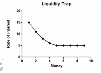
Liquidity Trap
Under the state of liquidity trap, the interest
rate is so low that the demand for money
becomes infinitely elastic. Moreover, the
supply of money will not affect the rate of
interest and income.
Baumol’s Inventory Theoretic Approach:
The theory was given in Baumol’s famous work “The Transaction Demand for Cash and
Inventory Theoretic Approach” in 1952.
Keynes → Mt,Mp, Msp Separately
Baumol → Together as Real cash Balance
Keynes → Demand for money = f (Y, i)
Baumol: Demand for money = f (Y, I, cost of transforming real cash balance into interest bearing
bonds)
Keynes → Mt is not a f (interest)
Baumol → Mt = f (interest).
❑ In short, in the theory given by Baumol, individuals hold money as a form of inventory
optimum cash holding. Opportunity cost of holding money is the interest income foregone.
❑ If interest rate on assets increase, then people readjust their portfolio by transferring money
towards those assets.
❑ Overall, individuals would hold money in the form in which their cost is minimum.
Costs of individual consist mainly of two; 1. Interest income foregone 2. Brokerage fee(b)
If b is very high, then the individual demands more money.
If r is high, then individual’s demand for money is less.
Friedman’s Restatement of Quantity Theory of Money:
The theory is based on the Cambridge’s quantity theory of money. It is also known as the
‘Modern Theory of Demand’ or ‘Capital Theoretic Approach’.
Friedman treats money as a capital good
Further, he stated that k is a function of:
a. rm (Rate of interest on income)
b. rb (Rate of interest on bonds)
c. re (Rate of interest on equities)
➢ Demand for money is the function of;
1. Rate of interest on income 2. Rate of interest on bonds 3. Rate of interest on equities
4. Wealth (W) 5. Proportion of Human to Non-Human Wealth (H)
6. Price Level (P) 7. Rate of Inflation Rate of interest

Tobin’s Theory of Interest Elasticity of Transaction Demand for cash:
❑ The theory was given in 1956. It is based on the Liquidity Preference Behavior towards risk. The
theory, unlike the previous ones, considers both risk and return.
❑ People want to maximise utility which is function of wealth and risk.
❑ Keynes: Individual held money either in the form cash or bond
Tobin: Individuals can hold both cash and bonds
Baumol-Tobin Theory:
❑ Baumol and Tobin together gave a theory for demand for money to prove that income
elasticity for demand for money is less than one; and change in demand for money is less than
the change in income
According to them, Bond Holding = f (Income, number of bond transactions)
Revenue = rate of interest * ABH (Average Bond Holding)
❑ When r increases, cash holdings decreases and people prefer to keep money in the banks, and
thus demand for money decreases.
❑ When Income increases, both bond holdings and cash holdings increase. However, increase in
cash holding is less than the increase in bond holdings. This implies that income elasticity of
demand for money is less than one.
❑ Empirically they calculated the values as:
Income elasticity for demand for money 0.5
Interest elasticity 0.5
QUESTIONS FOR CLARIFICATION
1. The word economy comes from the Greek word for
(a) environment.
(b) one who participates in a market.
(c) one who manages a household.
(d) conservation.
2. In the circular-flow diagram,
(a) firms are buyers in the product market.
(b) households are sellers in the resource market.
(c) firms are sellers in the resource market and the product market.
(d) spending on goods and services flow from firms to households.
3. An increase in the growth rate of the money supply is most likely to be followed by
a. a recession. b. inflation.
c. a decline in economic activity. d. all of the above.
4. Budget deficits can be a concern because they might
a. ultimately lead to lower inflation.
b. lead to lower interest rates.
c. lead to a higher rate of money growth which causes inflation.
d. cause all of the above to occur.
5. Which of the following are true statements?
a. Inflation is defined as a continual increase in the money supply.
b. Inflation is a condition of a continually rising price level.
c. The inflation rate is measured as the rate of change in the aggregate price level.
d. Only (b) and (c) of the above are true statements.
6. Assuming that the inflation rate is positive, which of the following statements characterizes the
relationship between the actual or observed interest rate and the real interest rate?
a. real interest rates are lower than actual interest rates
b. real interest rates are higher than actual interest rates
c. they are the same thing
d. none of the above is necessarily true
Answers:-
1)C 2)B 3)B 4)C 5)D 6)A
INVESTMENT THEORIES
❑ Financial Investments: Shares and bonds, etc. There is no addition or creation of capital
❑ Real Investment: It implies addition in capital stock
Fixed Invt.: Example, Machinery
Residential Invt.: Example, Housing
Inventory Invt.: Adding stock of capital
Keynes Theory of Investment
Keynes in his theory talks only about Real Investment.
Also, investment can either be autonomous (independent of level of income) or induced (function
of income). Therefore, Keynes gave the Investment function as follows:
I = f (MEC, r, business expectations)
MEC refers to the expected rate of return from investment over its cost.
Rate of Interest has a negative relation with that of investment.
There were two views about MEC;
❑ First view was given by Fischer who in 1963 stated that MEC is dependent on the profit
generated.
❑ Second view was given by Keynes who said that MEC is dependent on the expected return. It is
the rate of discount which would make prospective yield equal to its supply price, that is, which
makes return = cost.
According to Keynes, while considering MEC, rate of interest is relatively sticky.
Moreover, MEC declines with increase in investment because of two reasons:
a. Prospective yield with time decreases.
b. Supply price increases.
If MEC > r Investors will invest
If MEC < r Investors will not invest
So equilibrium is attained when MEC = r
Marginal Efficiency of Investment (MEI):
It reveals investments at different rates, given the optimal stock.
MEI curve shows the investment demand for the entire community at different rates of interest.
Accelerator Theory
❑ Clark gave the accelerator principle and this theory was propounded way before Keynes.
Before studying the accelerator theory, we need to understand the idea behind multiplier and
accelerator
Multiplier Change in investment leads to a change in income
Accelerator Change in income leads to a change in investment.
It/Δy = v = Accelerator
where, It: Level of Invt. ΔY: Changes in Income v: Accelerator
Acceleration theory of Investment describes a technological relationship between the change in
capital stock & the change in level of output.
Assumptions:
1. C-D production function 2. Factors of production are homogenous & perfectly divisible
3. Factor market is competitive & factor prices are given
4. Firms produce with least cost combination of inputs 5. No excess production capacity
6. Firms’ calculation about the future demand is fairly accurate
7. No financial constraint & funds are easily available
Fixed Accelerator Model: Assumptions of the model are:
• Accelerator (v) will be fixed
• No time lags in Investment decisions
• Instantaneous adjustment
• Excess capacity in Investment sector, that is, unutilized capital stock.
Flexible Accelerator Model:
It considers both optimal (desired) capital stock and Actual capital stock and there is a gap
between them.
Kt+1 – Kt = λ (K* - Kt)
Where: λ = speed of adjustment, K* = optimal capital stock
However, there is just partial fulfilment in the gap.
Moreover, λ is negatively affected by the rate of interest.
Investment are less volatile.
Capital Stock Adjustment:
• There are lags present. • Gap between optimal and actual is to be filled.
• Immediate adjustment would be more costly. • Per period addition is made.
Neo-Classical or Jorgenson’s theory of Investment:
The theory helps determine the desired level of capital that any firm would want to hold. The
theory used a Cobb-Douglous Production function.
Assumptions of the model:
a. Capital units are homogenous. b. No uncertainties. c. No adjustment costs.
d. Investment decisions are flexible before and after the decisions are taken.
e. Marginal productivity of labour and capital are positive.
y = AK^αL^1-α
Equilibrium would be attained were MPK = r/P
Where, r = rental, P = Price Level, and r/P = user cost
If MPK > r/P Invest
If MPK < r/P Not invest
Tobin’s Q Theory:
The theory was given in 1969.
𝐓𝐨𝐛𝐢𝐧 𝐐 = 𝐌𝐚𝐫𝐤𝐞𝐭 𝐯𝐚𝐥𝐮𝐞 𝐨𝐟 𝐢𝐧𝐬𝐭𝐚𝐥𝐥𝐞𝐝 𝐜𝐚𝐩𝐢𝐭𝐚𝐥 / 𝐑𝐞𝐩𝐥𝐚𝐜𝐞𝐦𝐞𝐧𝐭 𝐯𝐚𝐥𝐮𝐞 (𝐜𝐨𝐬𝐭)
If Q > 1 Invest because market valuation is higher
If Q < 1 Disinvest because cost is higher
Cash Flow Theory: Given by Duessenberry
MULTIPLIER
The first concept of multiplier was given by R.F. Kahn in 1931, namely Employment
Multiplier. Employment multiplier shows the impact on total employment with increase in
primary employment.
Investment Multiplier
The concept was given by Keynes and is also known as ‘Closed Economy Multiplier’. The
investment multiplier shows the change in income due to change in investment.
According to Keynes, repeated investment needs to be done.
Assumptions taken by Keynes were:
1. MPC constant 2. Closed economy
3. Ignored induced investment and accelerator effect.
4. Excess capacity in consumer goods industry.
5. No excess capacity in production sector.
Main features of investment multiplier are:
1. Higher MPC implies higher value of multiplier.
2. Multiplier can reduce due to leakages like savings, government taxes, imports, etc.
3. Value of the multiplier lies between 1 and infinity.
Foreign Trade Multiplier
The foreign trade multiplier implies that with increase in exports, what is the impact on income,
that is by how much does the income increase.
𝐅𝐨𝐫𝐞𝐢𝐠𝐧 𝐓𝐫𝐚𝐝𝐞 𝐌𝐮𝐥𝐭𝐢𝐩𝐥𝐢𝐞𝐫 = Δ𝐘 / Δ𝐗 = 𝟏 / 𝐌𝐏𝐌 + 𝐌𝐏𝐒
❑ Keynes Multiplier > Foreign Trade Multiplier
Super Multiplier
The concept of Super Multiplier was given by Hicks.
He considered both induced and autonomous investment.
Change in autonomous investment→ Change in income →Change in induced investment
I = A + iy
Where i = propensity to invest, A is the Autonomous investment, y = income.
𝐌𝐮𝐥𝐭𝐢𝐩𝐥𝐢𝐞𝐫 = 𝟏 / 𝐌𝐏𝐒 − 𝐌𝐏𝐈
Where: MPI = Marginal Propensity to Invest
❑ Super Multiplier > Investment Multiplier
Balanced Budget Multiplier
• Taxes are only autonomous and lump sum.
• Government purchases of goods and services are included and not the transfer payments.
• Government expenditure and tax do not affect the investment activity.
1. Government Purchases Multiplier: It reflects the change in income due to change in
government expenditure.
Δ𝐘 / Δ𝐆 = 𝟏 / 𝟏 − 𝐛
Where b = MPC
2. Tax Multiplier: It reflects the change in income due to change in taxes.
Δ𝐘 / Δ𝐓 = −𝐛 / 𝟏 − 𝐛
❑ Taxes imposed will reduce the consumption partially.
❑ Tax Multiplier < Government Multiplier
3. Balanced Budget Multiplier
𝐁𝐚𝐥𝐚𝐧𝐜𝐞𝐝 𝐁𝐮𝐝𝐠𝐞𝐭 𝐦𝐮𝐥𝐭𝐢𝐩𝐥𝐢𝐞𝐫 = 𝐆𝐨𝐯𝐞𝐫𝐧𝐦𝐞𝐧𝐭 𝐦𝐮𝐥𝐭𝐢𝐩𝐥𝐢𝐞𝐫 + 𝐓𝐚𝐱 𝐌𝐮𝐥𝐭𝐢𝐩𝐥𝐢𝐞𝐫
𝟏 /𝟏 − 𝐛 + −𝐛 /𝟏 − 𝐛 = 𝟏
Transfer Payments Multiplier = 𝒃 / 𝟏−𝒃
❑ Balanced budget multiplier is equal to one only in case of lump sum taxes. In case of
proportional tax, the balanced budget multiplier is less than 1.
TRADE CYCLES
• Trade Cycles are the alternate phases of business activity.
• They are universal, periodic and synchronous in nature.
• Profits are majorly affected by Trade cycles.
Boom: It is the peak level, that is, the topmost level
of expansionary phase. The economy experiences this
phase when it has crossed the full employment level.
At one side, when the economy shows signs of
prosperity, on the other hand, boom is a symptom
of downswing.
Recession (Upper turning point): The stage lies between
prosperity and depression. The process followed under this is:
Increase in interest rate → Decrease in Investment → Decrease in Income
→ Shut down the production
Theories of Trade Cycle
1. Samuelson’s Theory of Trade Cycle: The theory was given in 1939. Samuelson used the
concepts of both multiplier and accelerator.

❑ According to him,
Increase in autonomous investment → Increase in income (due to effect of multiplier)
→ Increase in induced investment (due to the effect of accelerator)
❑ According to Samuelson, cycles can be explosive in nature. He assumed different values of
multiplier and accelerator and considered a one period lag. Also he treated MPC to be
constant.
❑ Samuelson talked about 4situations:
1. Cycleless Growth Path: It goes away from the equilibrium path, either in increasing direction
or decreasing direction. MPC = 0.5 Accelerator = 0
2. Damped Fluctuations/ Oscillations: Magnitude is decreasing. It is not consistent with real
situations. MPC = 0.5 and Accelerator = 1
3. Constant Amplitude Cycle: It is not realistic.
MPC = 0.5 and Accelerator = 2
4. Anti-damped/ Explosive Cycles: It assumes no buffers could control the cycles.
MPC = 0.5 and Accelerator = 3
Hicks’ Theory of Trade Cycle:
The theory was given in 1950 in Hicks work namely “A Contribution to the Theory of Trade
Cycles”.
❑ His theory is also known as “Constrained Cycles Theory”. He used buffers in his theory and
stated that both the multiplier and the accelerator will lead to the generation of cycles.
❑ However, according to him, the explosive cycles can be controlled, which was not given in the
theory by Samuelson.
Where:
Max Y = Full employment ceiling level Y* = Equilibrium
growth path
Min Y = Floor ceiling/ slump equilibrium
I0ent = Autonomous Investment: It is determined by
capital stock. It determined the quantum of labour with
the help of multiplier.
Growth path would be determined by multiplier and accelerator.

In the diagram, movement from:
1 to 2: Expansion
2 to 3: Boom (Investment lag): Investment lag occurs because investment does not increase with
that pace as compared to the Growth path
3 to 4: Recession
5 to 6: Depression (represents excess capacity)
6 to 7: Recovery
Kaldor’s Theory “A model of Trade Cycle”: The theory was given in 1940. Kaldor uses the
concepts of savings and investment in the ex-ante form. He assumes a non-linear saving and
investment curve because they cannot be treated as constant. Moreover, with linear functions, the
trade cycles won’t be reflected.
Kaldor also stated that trade cycles are self-generating.
❑ Points b, c are the points of stable equilibrium and a is the
point of unstable equilibrium.
❑ Expansion process will generate when a and c are in the
process of co-incidence and will stop when these points coincide.

QUESTIONS FOR CLARIFICATIONS
1. Who first used the multiplier relationship together with the key role played by
unstable investment, which he expressed in terms of the accelerator theory of
investment to construct cumulative upwards and downwards movements in real
output?
A) Hicks B) Samuelson
C) Keynes D) Harrod
2.The effect of monetary and fiscal policies on private sector’s demand for goods
and financial assets must be taken into account if there is to be a complete and
consistent analysis of policy. This was first stated by:
A) D.J. Ott and A.F. Ott
B) D. Laldler and M. Parkin
C) G. Maynard and W.Van Ryckeghem
D) D. Purdy and G. Zis
3. Tinbergen rule of economic policy states that if government has ‘n’ independent
targets, it must then have at least ------- effective instrumental variables if it is to
achieve all the targets.
A) n-1 B) n+1 C) n+2 D) n
4. The new classical writers point to the repeated breakdown of econometric models
because:
A) Structural coefficients cannot be treated as invariant
B) Investment is related to interest rate
C) Existence of underemployment in the economy D) None of the above
5. Relative Income Hypothesis is propounded by:
A) M. Friedman B) J.M. Keynes
C) Duesenbery D) Modigliani
6. The cost of employing the services of a unit of capital includes:
A) Interest charged on the price of one unit of capital stock
B) Depreciation charge C) Rise in the price of a unit of capital stock
D) All the above
7. The stability of demand for money is seen as a crucial theoretical and empirical
idea for the:
A) Keynesians B) Post Keynesians
C) Monetarists D) New Keynesians
Answers:-
1) A 2) B 3) D 4) A 5) C 6) D 7) C
PHILLIPS CURVE
The concept of Phillips Curve was given by A.W. Phillips in 1958.
❑ Originally the relationship was estimated between wages and unemployment. It was stated
that there is a negative relationship between the two.
❑ If workers can push the wages beyond their productivity, then it will lead to the change in
price level.
Δ𝐖 / 𝐖 > Δ𝐲 / 𝐲
i.e., Δ𝐏 / 𝐏
❑ Later on, Phillips curve was established showing a negative relationship between rate of
inflation and rate of unemployment
• It is downward sloping and takes the shape of a rectangular hyperbola
Theoretical Explanations for trade-off between Rate of price level (ΔP/P) and Rate of
unemployment (ΔU/U)
1. Lipsey (1960): According to Lipsey, wages are directly related with excess demand.
Unemployment and excess demand are inversely related.
W = f (Nd – Ns)
Where: Nd = Demand for labour, Ns = Supply of labour,
Nd – Ns = Excess demand for labour, W = Wages.
2. Phelps: Phelps gave a theory named “Theory of Collective bargaining/ Trade Unionisation”.
❑ According to him, monetary settlements are through collective bargaining. Wages are
indirectly related to unemployment.
High unemployment rate →Less power with the trade union→ Decrease in wages
Keynes Dynamic analysis of price-output determination:
❑ According to Keynes, if there is an increase in aggregate demand, it will be distributed
between price level and unemployment. In other words, with increase in aggregate demand,
the price level will increase, while unemployment rate will decrease.
Policy Implications of Philips Curve
Expansionary: Increase in Inflation, Decrease in Unemployment
Contractionary: Decrease in Inflation, Increase in Unemployment
Long Run Phillips Curve
The Long-Run Phillips Curve was given by Milton Friedman.
It is also known as Augmented Phillips Curve or Adaptive Expectations Phillips Curve.
W = U + λPte
Where: W = Wages, U = Unemployment, λ = Speed of adjustment,
Pte = Price expectations.
λ = 1 would imply perfect expectations
λ = 0 in the short run
λ < 1, according to Tobin.
Natural Rate of Unemployment (NRU):
The concept of NRU was given by Milton Friedman while it was given a new name by Tobin which
is “Non-Accelerating Inflation Rate of Unemployment (NAIRU)”.
It is the rate at which there is no gap between actual and expected inflation. In other words,
inflation is stable at that point.
❑ Suppose if we adopt expansionary policy. The
unemployment would reduce to U2 level and inflation
is 3.5%. So labour will demand wages according to 3.5%
because they haven’t realised the inflation. But when
they do, they demand higher wages and Phillips curve
would then shift to SRPC 2. Long run Phillips curve will
show that there is no trade off between inflation rate
and unemployment rate. Any change in the policy would
only lead to increase in the inflation rate.

Ekstein-Brinner’s Phillips Curve:
According to this, there is no trade-off till NAU but beyond that there is a trade-off.
Decrease in unemployment rate below the natural rate is possible only if there is a time lag
between money wages and price levels.
Stagflation is a situation in which prices increase without increase in employment and output
levels.
IS-LM MODEL
The IS-LM Model was given by Hicks and Hansen in 1937. It reflects on the simultaneous
integration of the two sectors.
Product Market
IS curve shows equilibrium in the product market.
All the points on the IS curve show Saving = Investment and Aggregate Demand = Aggregate
Supply. Also there is a negative relationship between rate of interest and income.
Fall in rate of interest-→ Increase in Investment→ Increase in Aggregate
Demand→ Increase in income
Slope of IS Curve depends upon:
1. Interest elasticity of Investment Demand:
Small changes in interest rates, lead to larger
changes in Investment. Higher the interest
elasticity of demand, flatter will be the IS curve
and vice versa.
2. Size of the multiplier: More the size of the
multiplier, flatter will be the IS curve and vice-versa.
❑ IS curve shifts when the autonomous elements
changes.

Money market
Money market equilibrium is represented by LM Curve. At all points on the LM curve, demand for
money is equal to the supply of money. We assume that the supply of money is exogenously
determined by the bank or Central authority.
We know that, Md = f (y, i)
Money demand is a function of income and rate of interest
i and y are positively related
❑ Increase in income →Demand for money increases
→Sell bonds, which reduces the price of bonds
→Because demand for bonds is now less, the interest
rate increases


Monetary Policy
❑ In the Keynesian range, monetary policy is
completely ineffective and will not change
the rate of interest.
❑ In the intermediate range, policy is less
effective than the classical range and more
effective than the Keynesian range.
❑ In the intermediate range, policy is less
effective than the classical range and more
effective than the Keynesian range.

Fiscal Policy
❑ In the Keynesian range, fiscal policy is
highly effective.
❑ In the Intermediate range, fiscal policy is
less effective as compared to the Keynesian
range and more effective as compared to
the Classical Range.
❑ In the Classical range, fiscal policy is totally
ineffective. Entire impact is on the rate of
interest and no change in income.

NATIONAL INCOME AGGREGATES
GDP → Total Production
GNP = GDP-Net income from Abroad (NFIA)
GDP MP = GNPMP - NFIA
GDP FC = GDPMP – Net Indirect Taxes Net Indirect Tax = Indirect Taxes – subsidies
NNPMP = GDP – Depreciation
NDP = GDP - Depreciation
Real Y = Current year NNP/Current year index 100 National Income = NNPFC
Private Income= National income – Income of Govt. Cos. Savings of Non- Dept. Enterprises +
Interest on National debt + Net Current transfers from Govt. + Net
current transfers from abroad.
Personal Income = Private Y- Undistributed profits of enterprises – Corp. Tax – retained
earnings of foreign Cos.
Personal Disposable Y = Personal income – Personal Income Taxes – Misc. Receipt of the Govt.
Admin. Depts.
QUESTIONS FOR CLARIFICATION
1. The long run relationship between inflation and interest rates is called:
A) Keynes Effect B) Pigou Effect
C) Fischer Effect D) Patinkin Effect
2. GDP at market prices:
A) Includes indirect taxes and subsidies
B) Excludes indirect taxes but includes subsidies
C) Includes indirect taxes and excludes subsidies
D) Excludes both indirect taxes and subsidies
3. The tendency of increase in government spending to cause reductions in private
investment spending is:
A) Crowding–in effect B) Crowding-out effect
C) Cross subsidization D) Fiscal effect
4. Which of the following is not a fiscal measure?
A) Public expenditure B) Interest rate
C) Tax subsidies D) Investment subsidies
5. In a simple Keynesian Model, the open economy multiplier:
A) Is smaller in value than closed economy multiplier
B) Is greater in value than closed economy multiplier
C) Is same as closed economy multiplier
D) Cannot be compared to closed economy multiplier
6. A positive relation between the growth of the population, employment and output on the
one hand and the growth of labour productivity on the other is:
A) Verdoorn’s Law B) Labour Surplus Theory
C) Optimum Population Theory D) Demographic Transition Theory
7. Which of the following statement is not correct?
A) The value of Lorenz ratio ranges in between zero to one
B) The value of HDI ranges in between zero to one
C) The value of PQLI ranges in between one to 100
D) The SLR of RBI ranges in between 5 to 15.
8. Demonstration effect means:
A) Effect of advertisement B) Imitating effect of consumption
C) Effect of entertainment D) Effect of an experiment
Answers:-
1) C 2) C 3) B 4) B 5) A 6) A 7) D 8) B
MONEY
Definition of money
Narrow definition Currency (C) + Demand Deposits (DD)
Broader definition C + DD + Time Deposits (TD)
Gurley-Shaw Approach
According to them, Time Deposit and savings deposit can be substituted
Money = weighted average of all the assets (Weights are given according to their liquidity)
Liquidity Approach/ Central Bank Approach
Given by Radcliff
Money = state of liquidity in the economy.
High powered money →
Currency issued by Central Bank and is supported by Reserves India Adopted Minimum Reserve
System in Oct. 1956
Minimum Reserve System:
Presently 200 crores
→ 115 crore in Gold and other in rupee securities
Measure of High Power Money ss in India
H = C + R + OD
Where, C= Currency held by public, R= Cash Reserves of Commercial Banks
DETERMINANTS OF MONEY SUPPLY
1. Required Reserve Ratio = Sum of currency in the hands of public (c) + Cash Holdings &
deposits at the Central Bank (R)
2. Level of Bank Reserves = reserve ratio Commercial Banks /Deposit Liabilities
3. Public’s Desire to hold currency & deposits
Measures of Money Supply
These measures were adopted by our economy in 1977.
M1 = C + DD + Other deposits
M2 = M1 + Savings with the post office
M3 = M1 + Time Deposits
M4 = M3 + Post office savings (excluding NSC)
Liquid Resources
L1 = New M3 + All deposits of Post Office savings Banks excluding NSCs.
L2 = L1 + Term deposits c term lending inst. & refinancing inst. + term borrowing by FIs.
L3 = L2 + Public deposits of non-banking financial inst.
Money Multiplier
M = mH
Where: M = money supply, m = money multiplier, H = High Powered money
M = C + DD
H = C + Reserves (R)
R = Required reserves + excess reserves
❑ Money multiplier ‘m’ tell us that with change in H, how much will the money supply in the
economy change.
Determinants of Money multiplier
𝐌/ 𝐇 = 𝐂 + 𝐃 / 𝐂 + 𝐑
1. C/D is the currency deposit ratio which has a negative relationship with the money supply.
2. R/D is the reserve deposit ratio and has a negative relation with the money supply.
3. Proximate/Ultimate factors: like CRR, SLR, affect C/D, R/D
Systems of Money
1. Barter System: Exchange in terms of goods which was known as commodity money.
Problems under this system was:
• No durability
• No portability
• Not homogenous
2. Metallic Coins: It is a full bodied money. Money value is equal to the intrinsic value or
commodity money.
3. Credit Money: Commodity value is nil. Money value if much greater than commodity value.
INFLATION
Creeping Inflation Around 3%
Trotting inflation/Crawling/ walking 3-7 percent or less than 10%
Running Inflation 10-20%
Hyperinflation/Runaway inflation Above 20%
Causes of Inflation
1. Excess demand: According to monetarists, with the increase in money supply, there would be
a rise in the price level.
On the other hand, Keynesians stated that price would rise only after demand reaches income.
2. Cost push inflation: Cost of production increases.
Studies with respect to trade union activities.
3. Profit-push inflation:
It is also known as Administered pricing inflation or pricing power inflation.
It is studied from the employer’s side who increase the price above the cost of production to
increase their own profits.
4. Structural inflation: It is caused due to rigidities in the economy.
5. Mark-up inflation: It was given by Professor Ackley.
Wages of workers are administered by labour and employers together.
Employers keep price above the cost. On the other hand, labour keeps a mark up of its wages
above their minimum living requirements.
6. Sectoral Inflation/Demand shift rigidities: It was given by Charles Schultz. Such kind of an
inflation is caused due to downward rigidities in wages. If there is excess demand, prices increase
and in case of deficient demand, prices decrease. Overall, the net result is the increase in price.
Open Inflation: In this, the government doesn’t interfere. Activities are left on the market forces.
Suppress Inflation: It is the case in which open inflation is controlled by the government by
imposing monetary or fiscal limits.
Reflation: Occurs at times of recession/depression.
Government adopts the policies to increase the prices.
Core inflation: Also known as underlying inflation.
It is the inflation not accounting for volatile price movements, particularly food
and energy prices.
Headline inflation/topline inflation: Includes all the volatile inflation. It accounts for
everything which affects the cost of living.
AGGREGATE DEMAND AND AGGREGATE SUPPLY
Aggregate Demand
The curve slopes downwards because:
1. Real Balance Effect: If there is a decrease in
price, people become better off and hence
demand more quantity.
2. Rate of interest effect: Decrease in price
→demand for money decreases →rate of
interest decreases →Investment increases
→Aggregate demand increases
3. Net export effect: Decline in price, leads to increase in exports and hence the aggregate
demand increases.
Aggregate Supply: Aggregate supply curve is upward sloping because of nominal wage
rigidities in the short run.

AD curve shifts due to changes in government expenditure, investment and net exports. On the
other hand, AS curve shifts due to change in technology, input prices, taxes or subsidies.
Sticky Wage Model: By Lucas
𝐲 = 𝐲̅ + 𝛂(𝐏 − 𝐏^𝐞)
y = aggregate output
𝑦̅̅= Potential GDP (Labour market equilibrium, that is, NRU achieved)
α = Rate at which output is changing with change in prices
P = Price level P^e = Expected Price level
❑ The aggregate supply curve is a vertical curve in the long run because the money wages are
not sticky then. They are rather flexible so they keep the real quantity constant.
❑ If money wages increase, prices also increase and hence relative quantities remain stable.
❑ In the long run, macro-economic equilibrium will be established where equality is achieved
between aggregate demand, short run aggregate supply and long run aggregate supply.
It is the point where:
1. Real GDP = Potential GDP
2. P = Pe
3. Actual unemployment rate = Natural
rate of Unemployment (NRU)
In long run, money wages help in establishing
equilibrium because they are flexible.
NRU = Structural unemployment + Frictional Unemployment
EFFECTIVE DEMAND
Point where AD curve intersects AS
Effective demand determines the level of income & employment. Lack of effective demand →
unemployment.

Total effective demand includes :-
1. demand for consumption goods or consumption demand.
2. Demand for capital goods or Investment demand
Increase in consumption demand > Increase in total income → unemployment.
PATINKIN’S INTEGRATION OF MONETARY AND VALUE THEORY
THE REAL BALANCE EFFECT
Work “Money, Interest & Prices” : Book by Don Patinkin
❑ According to the theory, Demand & supply of goods are affected only by relative prices.
Money prices have no effect on demand & supply of goods implying Demand & supply
functions for goods are homogenous of degree zero. When prices level changes, purchasing
power of cash holdings will also changes which affects demand and supply of goods.
❑ This process is known as the REAL BALANCE EFFECT.
❑ Increase in price level →Decrease in real balance →Increase in Demand
PARADOX OF THRIFT
People save → Decrease in Consumption → Decrease in Standard of living.
This leads to decrease in economic growth Deposit multiplier = (1/r)*(D) ,
where D = Deposits of the Bank and
r = Required cash reserve ratio
FUNCTIONS OF MONEY
Primary functions Secondary functions Contingent functions
1. Medium of exchange Std. of deferred payment Distribution of NY
2. Medium of exchange Store of value Equating of MU
3. Measure of value Transfer of value Basis of credit
Liquidity to Wealth
QUESTIONS FOR CLARIFICATION
1. Negative net work externality in which a consumer wishes to own an exclusive or unique good
A) Demonstration Effect B) Ratchet Effect
C) Pigou Effect D) Snob Effect
2. Tobin’s Q is positive when the revenue from a unit of output produced by hiring
additional capital is -------
A) greater than the rental on capital.
B) lower than the rental on capital.
C) equal to the rental on capital.
D) None of the above
3. The demand for real money balances ----- with income and ----- with a rise in
interest rates
A) declines, rises B) rises, rises
C) declines, declines D) rises, declines
4. The assumption that money wages are fixed and that employment is determined by the short
side of the labour market, which is usually the demand for labour side results in
A) A downward sloping aggregate supply of output curve
B) An upward sloping aggregate supply of output curve
C) A vertical aggregate supply of output curve
D) None of the above
5. Under the Keynesian policy analysis, fiscal policy multiplier is larger when:
A) The more interest elastic is the demand for money and less interest elastic is the demand for
investment goods
B) The less interest elastic is the demand for money and less interest elastic is the demand for
investment goods
C) The more interest elastic is the demand for money and more interest elastic is the demand for
investment goods
D) The less interest elastic is the demand for money and more interest elastic is the demand for
investment goods
6. An increase in taxes will shift the
A) IS curve to the right and increase both the interest rate and the level of income
B) IS curve to the left and decrease both the interest rate and the level of income
C) IS curve to the right and increase the level of income but decrease the interest rate
D) LM curve downward to the right and increase the level of income but decrease the interest rate
7. When the rate of inflation is declining, there is
A) Reflation B) Deflation
C) Disinflation D) None of the above
Answers:-
1) D 2) A 3) D 4) B 5) A 6) B 7) C